Slide 1: Course Template (Reminder)

Purpose: Keep the recurring template visible.

• Decision variables: what we can choose.
• Objective (loss): what we want to make small.
• Algorithm: how we update the variables.
• Diagnostics: what we plot or log.

Slide 2: Optimization Problem

Purpose: Define the object we solve.

Formula:

• Decision variable: $w \in \mathbb{R}$.
• Objective: $L:\mathbb{R}\to\mathbb{R}$.
• Feasible set: $C \subseteq \mathbb{R}$.
• Unconstrained case: $C=\mathbb{R}$.

Slide 3: A Simple Constraint

Purpose: See a concrete constrained example.

Formula:

• Feasible set is $[0,\infty)$.

Slide 4: Convex vs Nonconvex Losses (1D)

Purpose: Fix the two toy losses used throughout.

• Convex quadratic: $L_{\text{quad}}(w)=\tfrac{1}{2}(w-1)^2$.
• Double well: $L_{\text{dw}}(w)=\tfrac{1}{2}(w^2-1)^2$.
• The scaling $\tfrac{1}{2}$ is cosmetic.
• Nonconvexity is the default in modern ML.

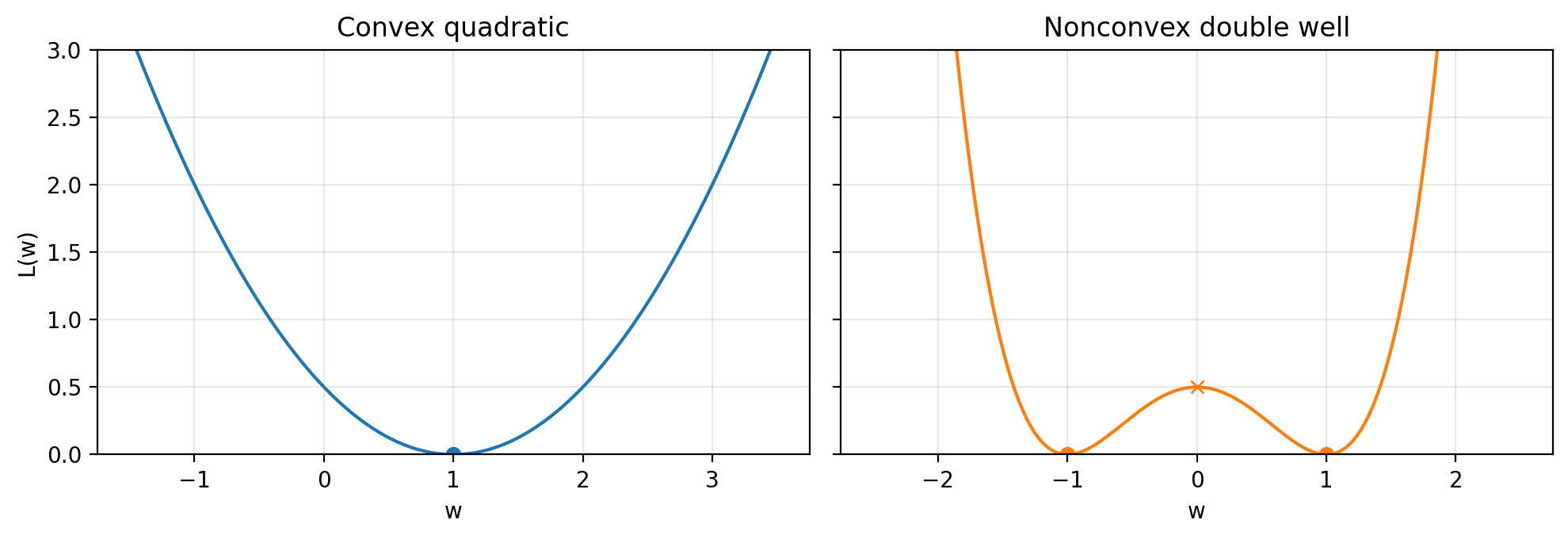Figure 1.1.

Slide 5: Global Minimizer

Purpose: Define what “minimizer” means.

Formula:

• $w^\ast$ must lie in $C$.

Slide 6: Optimal Value and Objective Gap

Purpose: Define the target value and a practical notion of “close.”

Formula:

• $L(w)-L^\ast$ is the objective gap (suboptimality gap).
• In toy examples, often $L^\ast=0$.

Slide 7: Stationary Points (Unconstrained)

Purpose: Define stationarity for differentiable, unconstrained problems.

Formula:

• Nonconvex problems can have many stationary points.

Slide 8: Constrained Stationarity (Preview)

Purpose: Flag what changes with constraints.

• Minimizers can sit on the boundary of $C$.
• Stationarity uses Lagrange multipliers.
• We return to this in a later lecture.

Slide 9: Iterative Algorithms

Purpose: Define what an iterative method produces.

Formula:

• Each $w_k$ is an approximate solution candidate.
• Main hyperparameter here: step size (learning rate) $\eta$.

Slide 10: Diagnostics

Purpose: Know what we monitor.

• Objective values: $L(w_k)$ (or $L(w_k)-L^\ast$ if $L^\ast$ is known).
• Gradient norm: $|L’(w_k)|$.
• Small gradients do not guarantee small objective.
• Example: for $L(w)=\tfrac{1}{2}(w^2-1)^2$ we have $L’(0)=0$ but $L(0)=\tfrac{1}{2}$.

Slide 11: Termination Criteria

Purpose: See standard stopping rules.

• Stop after a fixed number of iterations $T$.
• Stop when $|L’(w_k)| \le \varepsilon_{\text{grad}}$.
• Stop when $L(w_k)-L^\ast \le \varepsilon_{\text{obj}}$ (if $L^\ast$ is known).
• Stop when progress stalls (plateauing diagnostics).

Slide 12: What Makes an Algorithm “Good”

Purpose: Compare algorithms by resources.

• Memory: state stored per step (GD stores current iterate; others store history like momentum or quasi-Newton curvature).
• Computation: work per iteration.
• Computation: number of iterations to reach accuracy.
• Time-to-result: iterations to hit a target accuracy.

Slide 13: Iteration Counts and Rates

Purpose: Relate accuracy to iteration count.

Formula:

• Sublinear vs linear (geometric) decay.
• One might think “linear means a line.” However, it means geometric decay.

Slide 14: Semilog View of Convergence

Purpose: Visualize sublinear vs geometric decay.

• On a semilog-$y$ plot, geometric decay is a straight line.
• Sublinear decay bends.

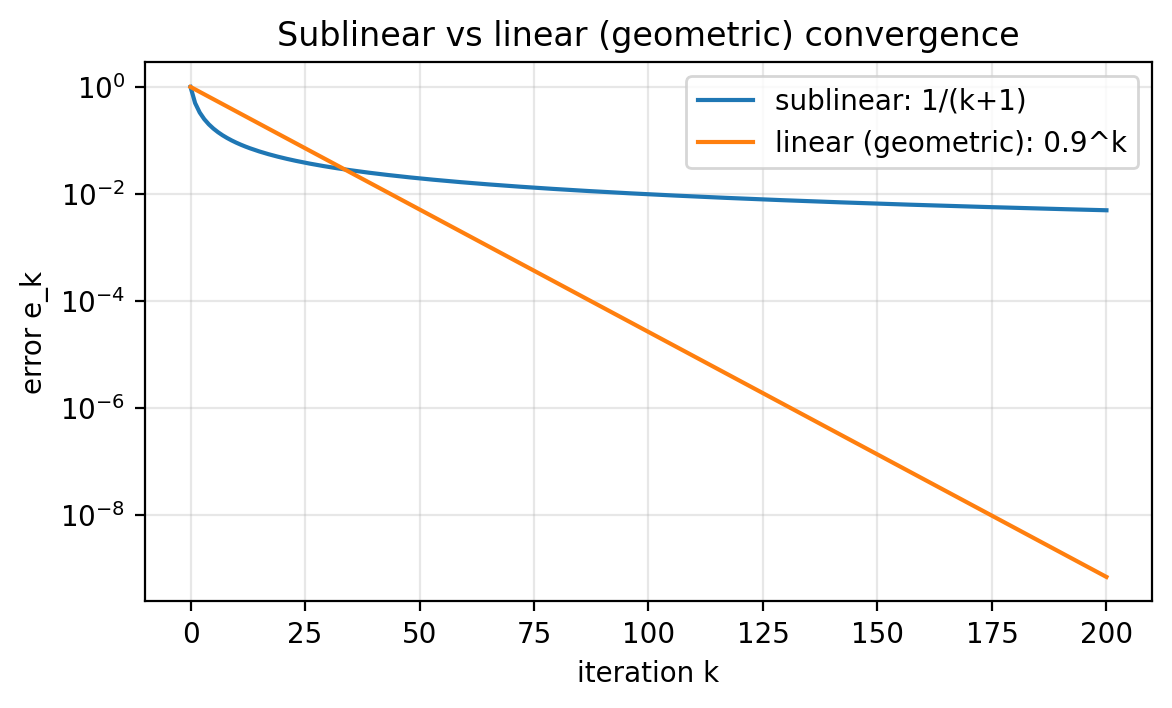Figure 1.2.

Slide 15: Local Model (Taylor)

Purpose: Motivate the descent direction.

Formula:

• The sign of $L’(w)$ tells which direction decreases the local model.

Slide 16: Gradient Descent Update (1D)

Purpose: State the update rule.

Formula:

• Move against the derivative to decrease the local model.

Slide 17: Local Decrease Check

Purpose: Show the first-order decrease.

Formula:

• For small enough $\eta$, the objective decreases to first order.
• In higher dimensions, $L’(w)$ becomes $\nabla L(w)$.

Slide 18: Quadratic Example for Code

Purpose: Fix the first objective for implementation.

Formula:

Slide 19: Minimal Loop Ingredients

Purpose: See the core steps of GD.

1. Initialize $w_0$.
2. Compute $L(w)$ and $L’(w)$.
3. Update $w \leftarrow w - \eta L’(w)$.
4. Log diagnostics.
5. Stop when a rule triggers.

Slide 20: Minimal Python Loop (Code)

Purpose: See the smallest runnable loop.

# Save as: script/gd_1d_python_minimal.py

def L(w: float) -> float:
    return 0.5 * w * w

def dL(w: float) -> float:
    return w

def main():
    w = 5.0
    eta = 0.5
    max_iters = 10

    for k in range(max_iters):
        Lw = L(w)
        gw = dL(w)
        print(f"k={k:2d}  w={w:+.6f}  L(w)={Lw:.3e}  |L'(w)|={abs(gw):.3e}")
        w = w - eta * gw

    print(f"final w={w:+.6f}  final L(w)={L(w):.3e}")

if __name__ == "__main__":
    main()

# Output:
# k= 0  w=+5.000000  L(w)=1.250e+01  |L'(w)|=5.000e+00
# k= 1  w=+2.500000  L(w)=3.125e+00  |L'(w)|=2.500e+00
# k= 2  w=+1.250000  L(w)=7.812e-01  |L'(w)|=1.250e+00
# k= 3  w=+0.625000  L(w)=1.953e-01  |L'(w)|=6.250e-01
# k= 4  w=+0.312500  L(w)=4.883e-02  |L'(w)|=3.125e-01
# k= 5  w=+0.156250  L(w)=1.221e-02  |L'(w)|=1.562e-01
# k= 6  w=+0.078125  L(w)=3.052e-03  |L'(w)|=7.812e-02
# k= 7  w=+0.039062  L(w)=7.629e-04  |L'(w)|=3.906e-02
# k= 8  w=+0.019531  L(w)=1.907e-04  |L'(w)|=1.953e-02
# k= 9  w=+0.009766  L(w)=4.768e-05  |L'(w)|=9.766e-03
# final w=+0.004883  final L(w)=1.192e-05

Slide 21: Full Python GD (Functions)

Purpose: Logging + stopping + diagnostics plot.

Logs $L(w_k)$ and $|L’(w_k)|$ each step; stops by eps_grad, eps_obj, or max_iters.

# Save as: script/gd_1d_python.py

import os
import matplotlib.pyplot as plt


def gradient_descent_1d(L, dL, w0, eta, max_iters=200, eps_grad=1e-8, eps_obj=None):
    """
    1D gradient descent with simple logging.

    Stops when:
      - k reaches max_iters, or
      - |L'(w)| <= eps_grad, or
      - L(w) <= eps_obj (if eps_obj is not None)

    Returns:
      w_final (float), hist (dict of lists)
    """
    w = float(w0)

    hist = {"k": [], "w": [], "L": [], "abs_dL": []}

    for k in range(max_iters):
        Lw = float(L(w))
        gw = float(dL(w))

        hist["k"].append(k)
        hist["w"].append(w)
        hist["L"].append(Lw)
        hist["abs_dL"].append(abs(gw))

        if eps_grad is not None and abs(gw) <= eps_grad:
            break
        if eps_obj is not None and Lw <= eps_obj:
            break

        w = w - eta * gw

    return w, hist


def save_diagnostics_plot(hist, outpath, title):
    k = hist["k"]
    Lvals = hist["L"]
    gabs = hist["abs_dL"]

    plt.figure(figsize=(6.5, 3.5))
    plt.semilogy(k, Lvals, label="objective L(w_k)")
    plt.semilogy(k, gabs, label="|L'(w_k)|")
    plt.xlabel("iteration k")
    plt.ylabel("value (semilog y)")
    plt.title(title)
    plt.grid(True, which="both", alpha=0.3)
    plt.legend()

    os.makedirs(os.path.dirname(outpath), exist_ok=True)
    plt.savefig(outpath, dpi=200, bbox_inches="tight")
    plt.close()

Slide 22: Full Python GD (Main + Output)

Purpose: End-to-end run and outputs.

def main():
    # Example: L(w) = 1/2 w^2, L'(w) = w
    def L(w): return 0.5 * w * w
    def dL(w): return w

    w0 = 5.0
    eta = 0.5

    w_final, hist = gradient_descent_1d(L, dL, w0=w0, eta=eta, max_iters=80, eps_grad=1e-10)
    print(f"Final w: {w_final:.6e}")
    print(f"Final L(w): {hist['L'][-1]:.6e}")
    print(f"Iterations: {len(hist['k'])}")

    save_diagnostics_plot(
        hist,
        outpath="figures/gd_python_quadratic_diagnostics.png",
        title="GD on L(w)=1/2 w^2 (pure Python)",
    )


if __name__ == "__main__":
    main()

# Output:
# Final w: 7.275958e-11
# Final L(w): 2.646978e-21
# Iterations: 37

Slide 23: Stopping Rule in the Example

Purpose: Make the output interpretable.

• Stop when $|L’(w)| \le 10^{-10}$ (eps_grad=1e-10).
• Max-iteration cap: 80.

Slide 24: Quadratic Diagnostics

Purpose: See objective and gradient decay together.

Formula:

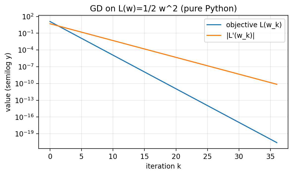Figure 1.3.

Slide 25: Changing the Loss Changes the Derivative

Purpose: See why hand derivatives do not scale.

• Shifted quadratic: $L(w)=\tfrac{1}{2}(w-1)^2$, $L’(w)=w-1$.
• Double well: $L(w)=\tfrac{1}{2}(w^2-1)^2$, $L’(w)=2w(w^2-1)$.
• Long compositions make mistakes more likely.

Slide 26: PyTorch Basics + Terminology

Purpose: Set the autodiff vocabulary.

• A tensor stores numbers; here $w$ is a scalar tensor.
• requires_grad=True tells PyTorch to compute $\frac{d}{dw} L(w)$ in w.grad.
• Forward pass: evaluate the loss.
• Backward pass: compute derivatives.

Slide 27: Single Derivative via backward()

Purpose: See autodiff on one scalar.

import torch

w = torch.tensor(2.0, requires_grad=True)  # track derivatives w.r.t. w
L = 0.5 * w**2                             # L(w) = 1/2 w^2

L.backward()                                # compute dL/dw

print("w =", w.item())
print("L =", L.item())
print("dL/dw =", w.grad.item())            # should be 2.0

# Output:
# w = 2.0
# L = 2.0
# dL/dw = 2.0

Slide 28: Sanity Check vs Analytic Derivative

Purpose: Verify autodiff on a known derivative.

import torch

def L_fn(w):
    return 0.5 * (w**2 - 1.0) ** 2

w = torch.tensor(2.0, requires_grad=True)
L = L_fn(w)
L.backward()

autograd_val = w.grad.item()
analytic_val = 2.0 * 2.0 * (2.0**2 - 1.0)   # 2w(w^2-1) at w=2

print("autograd:", autograd_val)
print("analytic:", analytic_val)

# Output:
# autograd: 12.0
# analytic: 12.0

Slide 29: Recorded Operations + Chain Rule

Purpose: Connect autodiff to calculus.

Formula:

• Example composition: $u(w)=w^2$, $v(u)=u-1$, $r(v)=\tfrac{1}{2}v^2$.
• Autodiff multiplies local derivatives automatically.

Slide 30: Forward Computation Sketch

Purpose: See the forward path for the example.

w  ->  u = w^2  ->  v = u - 1  ->  L = 0.5 * v^2

Slide 31: Backward Computation Sketch

Purpose: See local derivatives along the path.

L = 0.5 * v^2
  |  dL/dv = v
  v
v = u - 1
  |  d(v)/d(u) = 1
  v
u = w^2
  |  d(u)/d(w) = 2w
  v
  w

• Multiply local derivatives along the path to get $dL/dw$.

Slide 32: Pitfall A — Gradients Accumulate

Purpose: See why we must clear w.grad.

import torch

w = torch.tensor(2.0, requires_grad=True)

(0.5 * w**2).backward()
print("after first backward, w.grad =", w.grad.item())   # 2.0

(0.5 * (w - 1.0)**2).backward()
print("after second backward, w.grad =", w.grad.item())  # accumulated

w.grad = None
(0.5 * (w - 1.0)**2).backward()
print("after clearing, w.grad =", w.grad.item())         # correct for the last loss

# Output:
# after first backward, w.grad = 2.0
# after second backward, w.grad = 3.0
# after clearing, w.grad = 1.0

Slide 33: Pitfall B — Replacing the Tracked Variable

Purpose: See why the gradient disappears.

• Tempting update: w = w - eta * w.grad.

import torch

eta = 0.1
w = torch.tensor(2.0, requires_grad=True)

# Step 1
w.grad = None
L = 0.5 * w**2
L.backward()
print("step 1 grad:", w.grad.item())

# Wrong update: replaces the tracked variable
w = w - eta * w.grad

# Step 2
w.grad = None
L = 0.5 * w**2
L.backward()

print("step 2 grad:", w.grad)  # None because w is no longer the original tracked variable

# Output:
# step 1 grad: 2.0
# step 2 grad: None

Slide 34: Pitfall B — Correct Fix

Purpose: Update without tracking.

with torch.no_grad():
    w -= eta * w.grad

Slide 35: Pitfall C — Backward Twice

Purpose: Understand why reuse fails.

• The saved computation is cleared after the first backward pass.
• retain_graph=True keeps it, but we do not need it here.
• Standard loop: recompute loss each iteration, call backward() once, update.

Slide 36: PyTorch GD Loop (Function)

Purpose: The full autodiff loop structure.

# Save as: script/gd_1d_torch.py

import os
import torch
import matplotlib.pyplot as plt


def gd_1d_torch(L_fn, w0, eta, max_iters=200, eps_grad=1e-8, eps_obj=None):
    w = torch.tensor(float(w0), requires_grad=True)

    hist = {"k": [], "w": [], "L": [], "abs_dL": []}

    for k in range(max_iters):
        w.grad = None                 # clear accumulation

        L = L_fn(w)                   # forward pass
        L.backward()                  # backward pass

        g = w.grad.item()
        l = L.item()

        hist["k"].append(k)
        hist["w"].append(w.item())
        hist["L"].append(l)
        hist["abs_dL"].append(abs(g))

        if eps_grad is not None and abs(g) <= eps_grad:
            break
        if eps_obj is not None and l <= eps_obj:
            break

        with torch.no_grad():
            w -= eta * w.grad

    return w.item(), hist

Slide 37: PyTorch GD Loop (Plot Helper)

Purpose: Diagnostics plot helper.

def save_diagnostics_plot(hist, outpath, title):
    k = hist["k"]
    L_vals = hist["L"]
    gabs = hist["abs_dL"]

    plt.figure(figsize=(6.5, 3.5))
    plt.semilogy(k, L_vals, label="loss L(w_k)")
    plt.semilogy(k, gabs, label="|dL/dw at w_k|")
    plt.xlabel("iteration k")
    plt.ylabel("value (semilog y)")
    plt.title(title)
    plt.grid(True, which="both", alpha=0.3)
    plt.legend()

    os.makedirs(os.path.dirname(outpath), exist_ok=True)
    plt.savefig(outpath, dpi=200, bbox_inches="tight")
    plt.close()

Slide 38: PyTorch GD Loop (Main + Output)

Purpose: Run three losses with the same loop.

def main():
    w0 = 5.0
    eta = 0.5
    eta_dw = 0.02

    # Loss 1: quadratic
    def L1(w): return 0.5 * w**2
    w_final, hist = gd_1d_torch(L1, w0=w0, eta=eta, max_iters=80, eps_grad=1e-10)
    print(f"[quadratic]  final w={w_final:.6e}, final L={hist['L'][-1]:.6e}, iters={len(hist['k'])}")
    save_diagnostics_plot(hist, "figures/gd_torch_quadratic_diagnostics.png", "GD on L(w)=1/2 w^2 (PyTorch)")

    # Loss 2: shifted quadratic (no derivative code changes)
    def L2(w): return 0.5 * (w - 1.0) ** 2
    w_final, hist = gd_1d_torch(L2, w0=w0, eta=eta, max_iters=80, eps_grad=1e-10)
    print(f"[shifted]    final w={w_final:.6e}, final L={hist['L'][-1]:.6e}, iters={len(hist['k'])}")

    # Loss 3: double well (no derivative code changes)
    def L3(w): return 0.5 * (w**2 - 1.0) ** 2
    w_final, hist = gd_1d_torch(L3, w0=w0, eta=eta_dw, max_iters=200, eps_grad=1e-10)
    print(f"[doublewell] final w={w_final:.6e}, final L={hist['L'][-1]:.6e}, iters={len(hist['k'])}")


if __name__ == "__main__":
    main()

# Output:
# [quadratic]  final w=7.275958e-11, final L=2.646978e-21, iters=37
# [shifted]    final w=1.000000e+00, final L=0.000000e+00, iters=27
# [doublewell] final w=9.999991e-01, final L=1.818989e-12, iters=200

Slide 39: Autodiff Diagnostics

Purpose: See the same diagnostics with autodiff.

• Only the definition of L_fn changes.
• For the double well, we reduce the step size for stability.

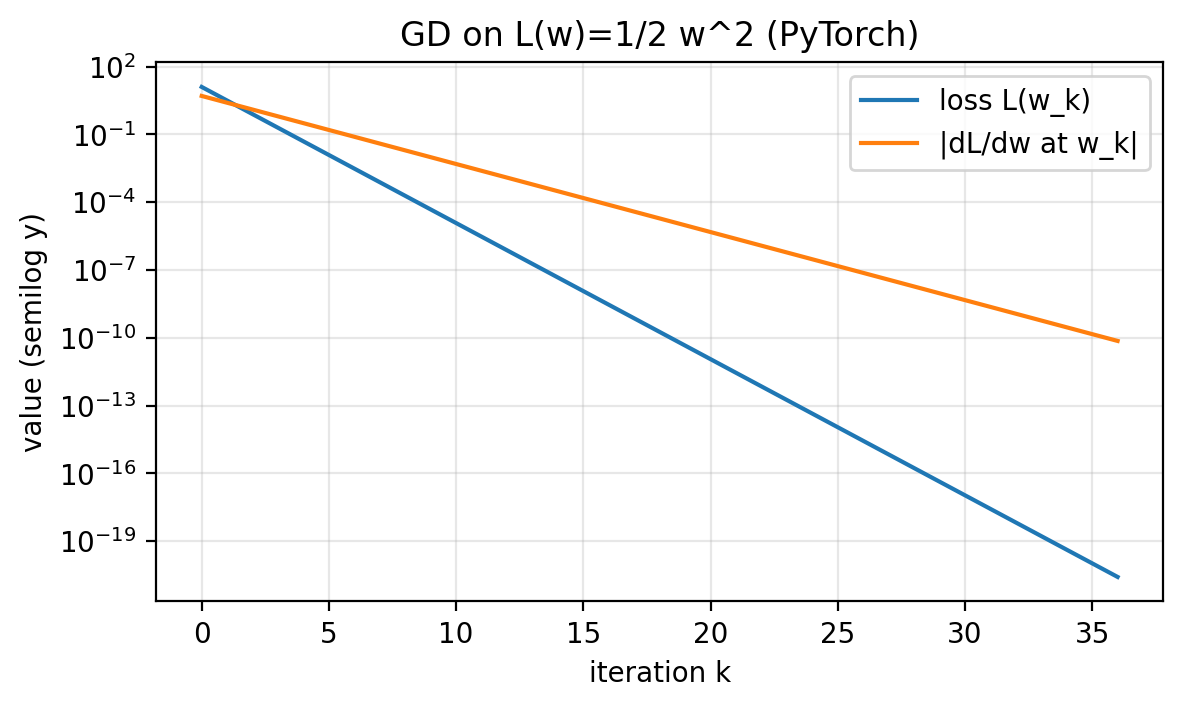Figure 1.4.

Slide 40: Step Size Tradeoff

Purpose: Understand the tuning tradeoff.

• Move aggressively (fewer iterations when stable).
• Avoid overshooting (divergence).

Slide 41: Quadratic Recursion and Stability

Purpose: Get exact behavior on the quadratic.

Formula:

• If $\eta=1$, then $w_1=0$ for any $w_0$.
• If $\eta=3$, then $w_{k+1}=-2w_k$ and $|w_k|$ doubles each step.

Slide 42: Step Size Comparison (Quadratic)

Purpose: See stable vs divergent behavior.

• $\eta=0.001$ (slow).
• $\eta=0.5$ (fast).
• $\eta=3$ (diverges).

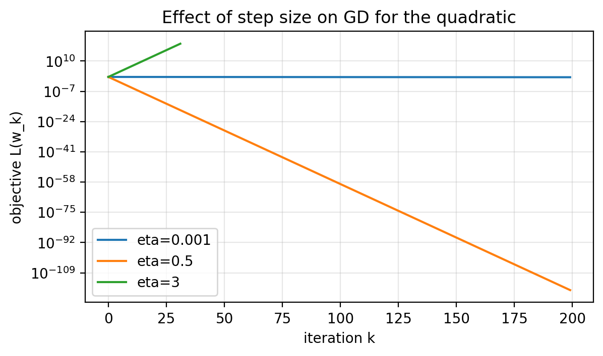Figure 1.5.

Slide 43: Time-to-Result Definition

Purpose: Define the tuning metric.

Formula:

• Time-to-result: iterations to hit the target (with a max-iteration cap).

Slide 44: Step Size Sweep (Quadratic)

Purpose: Choose a step size empirically.

• For this quadratic, the winner is near $\eta=1$.

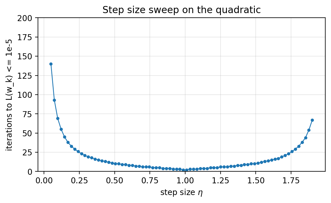Figure 1.6.

Slide 45: Nonconvex Sweep (Double Well)

Purpose: See how tuning depends on initialization.

Formula:

• Two global minimizers ($w=-1$ and $w=1$).
• Curvature depends on where you are.
• We use $w_0=2$ with a 2000-iteration cap (log $y$).
• Runs that miss the target hit the cap.

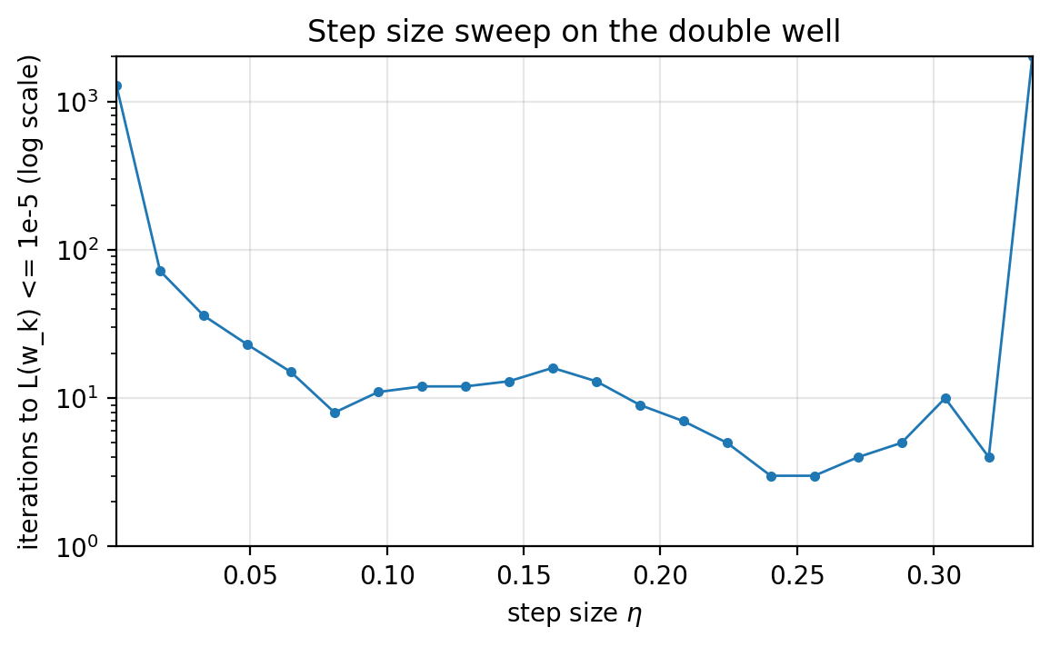Figure 1.7.

Slide 46: Conclusion

Purpose: Capture the main takeaways.

• An optimization problem = decision variable + objective + constraints.
• Minimizers and stationarity are different targets.
• Judge algorithms by diagnostics and time-to-result.
• Gradient descent comes from the local (Taylor) model.
• Autodiff avoids hand-derivative mistakes on long compositions.
• PyTorch loop rules: mark variables, clear w.grad, update under torch.no_grad().