1. Optimization and PyTorch Basics in 1D
Table of contents
- Setup: what is an optimization problem?
- Solutions, optimal values, and stationarity
- Iterative algorithms and diagnostics
- Gradient descent in 1D via the local model
- Implementation in NumPy: gradients by hand
- Implementation in PyTorch: gradients by
backward() - Autograd under the hood: recorded operations + chain rule
- Tuning: choosing a step size
- Conclusion
1. Setup: what is an optimization problem?
Reminder from last time:
- Decision variables: what we are allowed to choose.
- Objective (loss): what we want to make small.
- Algorithm: how we update the decision variables.
- Diagnostics: what we plot or log to see if the algorithm is behaving.
In this lecture we do everything in one dimension so that the objects are concrete.
Optimization problems
An optimization problem is:
\[\min_{w \in C} L(w)\]- Decision variable: $w \in \mathbb{R}$ (a number we choose).
- Objective / loss: $L:\mathbb{R}\to\mathbb{R}$ (a scalar function we can evaluate).
- Constraint set (feasible set): $C \subseteq \mathbb{R}$ (the allowed values of $w$).
Unconstrained problems are the special case $C=\mathbb{R}$:
\[\min_{w \in \mathbb{R}} L(w)\]A simple constrained example is a bound constraint:
\[\min_{w \ge 0} (w-1)^2\]Here the feasible set is $C=[0,\infty)$.
Convex vs nonconvex losses (in 1D)
Two toy losses we will use repeatedly:
- Convex quadratic:
- A nonconvex “double well”:
The scaling $\tfrac{1}{2}$ is cosmetic. It keeps some derivatives simple.
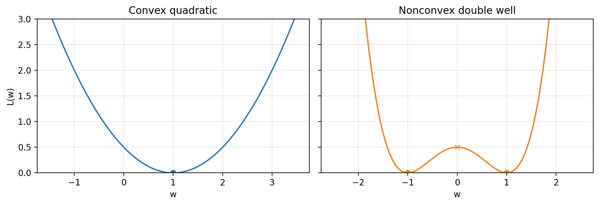 Figure 1.1: A convex quadratic (one minimizer) versus a nonconvex double well (two minimizers). Convexity is global geometry. Nonconvexity is the default in modern ML.
2. Solutions, optimal values, and stationarity
Minimizers and optimal value
A point $w^\ast$ is a (global) minimizer if $w^\ast \in C$ and
\[L(w^\ast) \le L(w) \quad \text{for all } w \in C\]The optimal value is
\[L^\ast = \inf_{w \in C} L(w)\]If a minimizer $w^\ast$ exists, then $L^\ast = L(w^\ast)$.
In many problems we care about approximate minimizers: points $w$ whose objective value is close to $L^\ast$. A standard definition is:
\[L(w) - L^\ast \le \varepsilon\]This quantity $L(w)-L^\ast$ is the objective gap (also called suboptimality gap). In real ML problems we typically do not know $L^\ast$, so the objective gap is not directly observable. In our toy 1D examples we often have $L^\ast=0$, so the objective gap is just $L(w)$.
Stationary points
For unconstrained problems with differentiable $L$, a stationary point is a point where the derivative is zero:
\[L'(w)=0\]An $\varepsilon$-stationary point is a point where
\[\|L'(w)\| \le \varepsilon\]It’s a bit more complicated to explain stationarity in constrained problems. Indeed, for constrained problems minimizers can occur at the “boundary” of constraint sets, and we need to introduce appropriate “lagrange multipliers” to quantify how “stationary” a given point is. We will leave this discussion. to another lecture.
Nonconvex problems can have many stationary points: local minima, local maxima, and flat points. In nonconvex ML, convergence guarantees often target stationarity rather than global optimality.
3. Iterative algorithms and diagnostics
Iterative algorithms
An iterative method produces a sequence
\[w_0, w_1, w_2, \dots\]Each $w_k$ is an approximate solution candidate. The algorithm usually has a small number of knobs (hyperparameters). In this lecture the main knob is the step size (learning rate) $\eta$.
What we monitor
Two common diagnostics are:
- Objective values: $L(w_k)$ (or objective gap $L(w_k)-L^\ast$ when $L^\ast$ is known).
- Gradient norm: in 1D this is $|L’(w_k)|$.
Since we’re trying to minimize $L$, we’d like it to decrease along the iterate sequence. If we also know $L^\ast$ we can also tell how well we’re solving the problem. However in general $L^\ast$ is not known, so we can never quite tell how well we’re solving the problem.
Gradient norms are a slightly weaker metric. For certain problems, we can show that whenever $|L’(w_k)|$ is small we also have that $L(w_k) - L^\ast$ is small. However, characterizing the precise relationship between the two is difficult and, in general, small gradients do not mean the objective is small. For example, for the double well $L(w)=\tfrac{1}{2}(w^2-1)^2$ we have $L’(0)=0$ but $L(0)=\tfrac{1}{2}$. On the other hand, gradients are at least always computable and always tend to zero as our iterates approach minimizers, so they’re still a useful diagnostic.
Termination criteria
Common stopping rules:
- Stop after a fixed number of iterations $T$.
- Stop when $|L’(w_k)| \le \varepsilon_{\text{grad}}$.
- Stop when $L(w_k)-L^\ast \le \varepsilon_{\text{obj}}$ (only when $L^\ast$ is known).
- Stop when progress stalls (plateauing diagnostics).
In our toy problem we will combine a max-iteration cap with a threshold on either the objective or the gradient.
What makes an algorithm “good”?
Two basic resources:
- Memory. What state must be stored to take the next step?
- Gradient descent stores the current iterate (and maybe a few running statistics).
- Other methods may store a history (momentum, quasi-Newton curvature, etc.).
- Computation.
- Work per iteration: what does one step cost?
- Number of iterations: how many steps do we need to reach a target accuracy?
A useful way to talk about iteration counts is: to reach an accuracy $\varepsilon$, the algorithm needs $T(\varepsilon)$ steps. Typical scalings look like:
- Sublinear rates: $T(\varepsilon)$ behaves like a power of $1/\varepsilon$.
- Linear rates (optimization jargon): $T(\varepsilon)$ behaves like $\log(1/\varepsilon)$.
One might think “linear convergence means the error decays like a line.” However, in optimization, linear convergence means geometric decay.
A standard model for the error is:
- Sublinear decay:
- Linear (geometric) decay:
On a semilog-$y$ plot, geometric decay is a straight line. Sublinear decay bends.
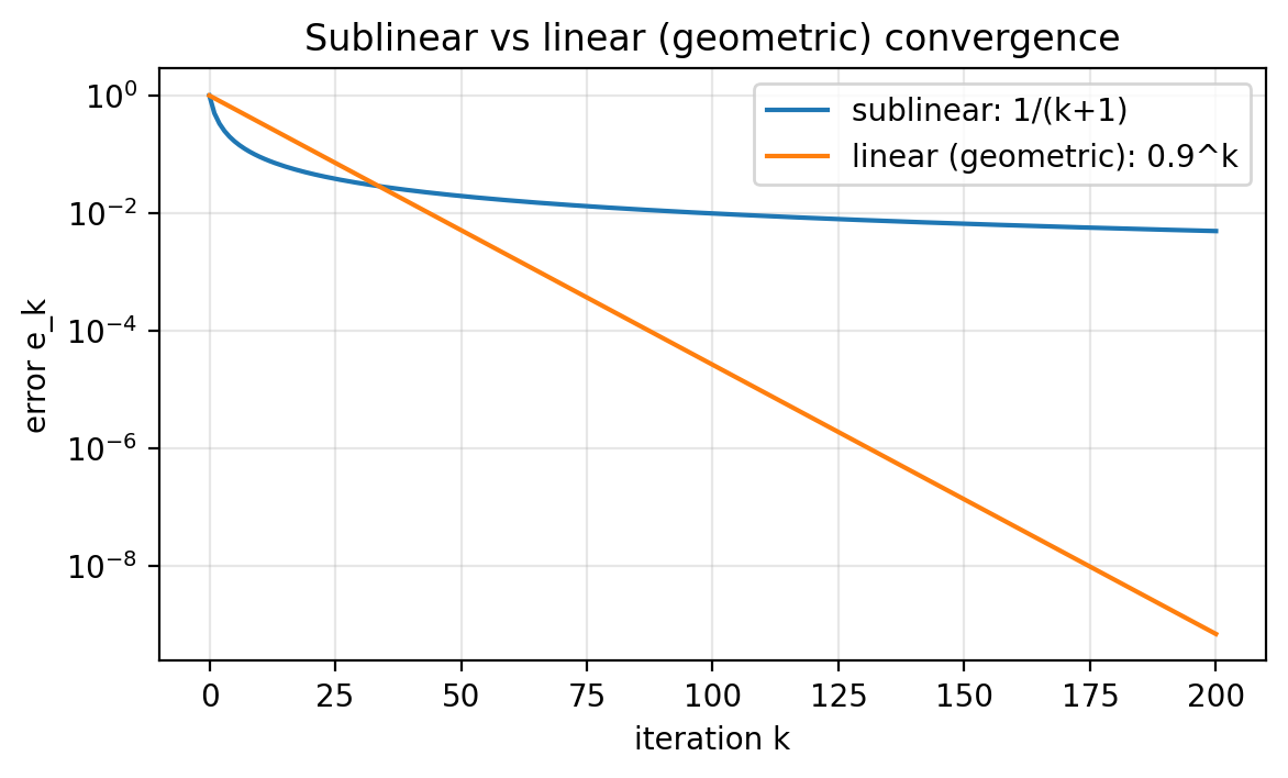 Figure 1.2: Semilog-$y$ plot of two toy error sequences. Geometric decay (called “linear convergence” in optimization) appears as a straight line. Sublinear decay bends.
4. Gradient descent in 1D via the local model
The local model (Taylor approximation)
Let $L:\mathbb{R}\to\mathbb{R}$ be differentiable. Near a point $w$, the first-order Taylor approximation is:
\[L(w+\Delta) \approx L(w) + L'(w)\Delta\]This approximation says: locally, $L$ looks like an affine function with slope $L’(w)$.
If $L’(w)>0$, then decreasing $w$ (negative $\Delta$) decreases the local model. If $L’(w)<0$, then increasing $w$ decreases the local model.
This motivates the gradient descent update.
Gradient descent update rule (1D)
Gradient descent with step size $\eta>0$ uses:
\[w_{k+1} = w_k - \eta L'(w_k)\]A basic check is to plug the update into the first-order model:
\[L(w_k - \eta L'(w_k)) \approx L(w_k) - \eta \|L'(w_k)\|^2\]So for small enough $\eta$, the objective decreases to first order.
In higher dimensions, $L’(w)$ becomes $\nabla L(w)$, and $|L’(w)|^2$ becomes $|\nabla L(w)|^2$. The mechanism is the same.
5. Implementation in pure Python: derivatives by hand
We will implement gradient descent using ordinary Python floats. In 1D, the loop is small enough that you can see every moving piece.
We will start with the quadratic objective
\[\begin{aligned} L(w) &= \tfrac{1}{2}w^2 \\ L'(w) &= w \end{aligned}\]A minimal gradient descent loop
A minimal loop has the following ingredients:
- Initialize a starting point $w_0$.
- Repeat:
- compute the loss $L(w)$,
- compute the derivative $L’(w)$,
- update $w \leftarrow w - \eta L’(w)$,
- log what happened (so you can debug and tune),
- stop when a rule triggers.
Minimal version: update + printing
# Save as: script/gd_1d_python_minimal.py

def L(w: float) -> float:
    return 0.5 * w * w

def dL(w: float) -> float:
    return w

def main():
    w = 5.0
    eta = 0.5
    max_iters = 10

    for k in range(max_iters):
        Lw = L(w)
        gw = dL(w)
        print(f"k={k:2d}  w={w:+.6f}  L(w)={Lw:.3e}  |L'(w)|={abs(gw):.3e}")
        w = w - eta * gw

    print(f"final w={w:+.6f}  final L(w)={L(w):.3e}")

if __name__ == "__main__":
    main()

# Output:
# k= 0  w=+5.000000  L(w)=1.250e+01  |L'(w)|=5.000e+00
# k= 1  w=+2.500000  L(w)=3.125e+00  |L'(w)|=2.500e+00
# k= 2  w=+1.250000  L(w)=7.812e-01  |L'(w)|=1.250e+00
# k= 3  w=+0.625000  L(w)=1.953e-01  |L'(w)|=6.250e-01
# k= 4  w=+0.312500  L(w)=4.883e-02  |L'(w)|=3.125e-01
# k= 5  w=+0.156250  L(w)=1.221e-02  |L'(w)|=1.562e-01
# k= 6  w=+0.078125  L(w)=3.052e-03  |L'(w)|=7.812e-02
# k= 7  w=+0.039062  L(w)=7.629e-04  |L'(w)|=3.906e-02
# k= 8  w=+0.019531  L(w)=1.907e-04  |L'(w)|=1.953e-02
# k= 9  w=+0.009766  L(w)=4.768e-05  |L'(w)|=9.766e-03
# final w=+0.004883  final L(w)=1.192e-05
Full version: logging + stopping + a diagnostics plot
This version logs $L(w_k)$ and $|L’(w_k)|$ each step and stops by eps_grad, eps_obj, or max_iters.
# Save as: script/gd_1d_python.py

import os
import matplotlib.pyplot as plt


def gradient_descent_1d(L, dL, w0, eta, max_iters=200, eps_grad=1e-8, eps_obj=None):
    """
    1D gradient descent with simple logging.

    Stops when:
      - k reaches max_iters, or
      - |L'(w)| <= eps_grad, or
      - L(w) <= eps_obj (if eps_obj is not None)

    Returns:
      w_final (float), hist (dict of lists)
    """
    w = float(w0)

    hist = {"k": [], "w": [], "L": [], "abs_dL": []}

    for k in range(max_iters):
        Lw = float(L(w))
        gw = float(dL(w))

        hist["k"].append(k)
        hist["w"].append(w)
        hist["L"].append(Lw)
        hist["abs_dL"].append(abs(gw))

        if eps_grad is not None and abs(gw) <= eps_grad:
            break
        if eps_obj is not None and Lw <= eps_obj:
            break

        w = w - eta * gw

    return w, hist


def save_diagnostics_plot(hist, outpath, title):
    k = hist["k"]
    Lvals = hist["L"]
    gabs = hist["abs_dL"]

    plt.figure(figsize=(6.5, 3.5))
    plt.semilogy(k, Lvals, label="objective L(w_k)")
    plt.semilogy(k, gabs, label="|L'(w_k)|")
    plt.xlabel("iteration k")
    plt.ylabel("value (semilog y)")
    plt.title(title)
    plt.grid(True, which="both", alpha=0.3)
    plt.legend()

    os.makedirs(os.path.dirname(outpath), exist_ok=True)
    plt.savefig(outpath, dpi=200, bbox_inches="tight")
    plt.close()


def main():
    # Example: L(w) = 1/2 w^2, L'(w) = w
    def L(w): return 0.5 * w * w
    def dL(w): return w

    w0 = 5.0
    eta = 0.5

    w_final, hist = gradient_descent_1d(L, dL, w0=w0, eta=eta, max_iters=80, eps_grad=1e-10)
    print(f"Final w: {w_final:.6e}")
    print(f"Final L(w): {hist['L'][-1]:.6e}")
    print(f"Iterations: {len(hist['k'])}")

    save_diagnostics_plot(
        hist,
        outpath="figures/gd_python_quadratic_diagnostics.png",
        title="GD on L(w)=1/2 w^2 (pure Python)",
    )


if __name__ == "__main__":
    main()

# Output:
# Final w: 7.275958e-11
# Final L(w): 2.646978e-21
# Iterations: 37
Here we stop when $|L’(w)| \le 10^{-10}$ (set by eps_grad=1e-10), with a max-iteration cap of 80.
For $L(w)=\tfrac{1}{2}w^2$, the objective and the derivative are directly related:
\[L(w)=\tfrac{1}{2}w^2=\tfrac{1}{2}\,|L'(w)|^2\]So stopping by small objective and stopping by small derivative are closely aligned in this specific example.
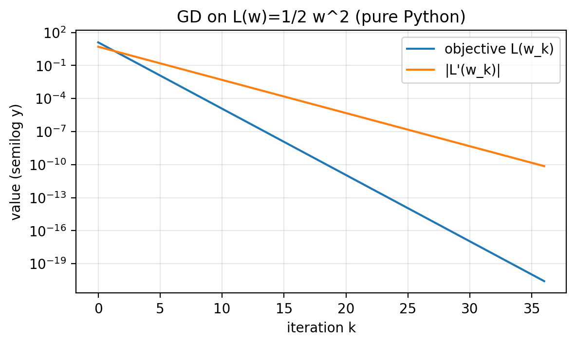 Figure 1.3: On the quadratic, both the objective and the derivative magnitude decay geometrically when the step size is stable.
Changing the loss means changing the derivative
A hand-written loop hard-codes two ingredients:
- how to compute the loss $L(w)$,
- how to compute the derivative $L’(w)$.
If you change the loss, you must update both.
Two examples:
- Shifted quadratic:
- Double well:
For simple formulas this is manageable. As soon as the loss becomes a long composition of operations, it becomes easy to make a mistake. That is where automatic differentiation becomes valuable.
6. PyTorch basics: tensors, requires_grad, and backward()
PyTorch can compute derivatives automatically. You write the loss as code, and PyTorch produces the derivative with respect to variables you mark as trackable.
In such (reverse mode) autodifferentiation software, we call the evaluation of the loss function on a given input a forward pass. We call the computation of the derivative, on the other hand, the backward pass.
In this lecture we will treat a single scalar $w$ as our parameter. In PyTorch, even a scalar is represented as a tensor.
What is a tensor here?
A tensor is a container for numbers. In this section:
wwill be a scalar tensor (think: “a number with extra bookkeeping”),- we will ask PyTorch to store $\frac{d}{dw} L(w)$ in
w.grad.
A single derivative via backward()
import torch

w = torch.tensor(2.0, requires_grad=True)  # track derivatives w.r.t. w
L = 0.5 * w**2                             # L(w) = 1/2 w^2

L.backward()                                # compute dL/dw

print("w =", w.item())
print("L =", L.item())
print("dL/dw =", w.grad.item())            # should be 2.0

# Output:
# w = 2.0
# L = 2.0
# dL/dw = 2.0
What to remember:
requires_grad=Truetells PyTorch to compute derivatives with respect tow.L.backward()computes the derivative and stores it inw.grad.w.gradis a tensor;.item()turns it into a Python float for printing.
Sanity check (recommended before writing any loop)
Compare to an analytic derivative at one point.
For the double well,
\[\begin{aligned} L(w) &= \tfrac{1}{2}(w^2-1)^2 \\ L'(w) &= 2w(w^2-1) \end{aligned}\]import torch
def L_fn(w):
return 0.5 * (w**2 - 1.0) ** 2
w = torch.tensor(2.0, requires_grad=True)
L = L_fn(w)
L.backward()
autograd_val = w.grad.item()
analytic_val = 2.0 * 2.0 * (2.0**2 - 1.0) # 2w(w^2-1) at w=2
print("autograd:", autograd_val)
print("analytic:", analytic_val)
# Output:
# autograd: 12.0
# analytic: 12.0
This is a quick consistency check before you write a full loop.
7. Autodiff under the hood, common pitfalls, and the training loop
Recorded operations + chain rule (what backward() is doing)
When you compute a loss from w, PyTorch records the sequence of operations used to build that loss. During backward(), it applies the chain rule in reverse order.
That is why it is called “backward”: the chain rule starts at the end (the loss) and works back through the computation.
Example loss:
\[L(w)=\tfrac{1}{2}(w^2-1)^2\]One way to view this as a composition:
- $u(w)=w^2$
- $v(u)=u-1$
- $r(v)=\tfrac{1}{2}v^2$
Then $L = r \circ v \circ u$, so
\[L'(w)=r'(v(u(w)))\,v'(u(w))\,u'(w)\]PyTorch performs this same multiplication of local derivatives, but it does it automatically from the recorded operations.
A sketch of the forward computation:
w -> u = w^2 -> v = u - 1 -> L = 0.5 * v^2
A sketch of the backward computation (same example, with local derivatives):
L = 0.5 * v^2
  |  dL/dv = v
  v
v = u - 1
  |  d(v)/d(u) = 1
  v
u = w^2
  |  d(u)/d(w) = 2w
  v
  w
To read it: multiply the local derivatives along the path to get $dL/dw$.
Pitfall A: gradients accumulate unless you clear them
If you call backward() multiple times, PyTorch adds into w.grad. For “one gradient per step” loops, you must clear w.grad each iteration.
import torch

w = torch.tensor(2.0, requires_grad=True)

(0.5 * w**2).backward()
print("after first backward, w.grad =", w.grad.item())   # 2.0

(0.5 * (w - 1.0)**2).backward()
print("after second backward, w.grad =", w.grad.item())  # accumulated

w.grad = None
(0.5 * (w - 1.0)**2).backward()
print("after clearing, w.grad =", w.grad.item())         # correct for the last loss

# Output:
# after first backward, w.grad = 2.0
# after second backward, w.grad = 3.0
# after clearing, w.grad = 1.0
Pitfall B: tracking the update step breaks the loop
A tempting update is:
w = w - eta * w.grad
This creates a new w and replaces the original tracked variable. PyTorch only fills .grad for the original variable you told it to track, so after the replacement, w.grad is empty in the next step.
A tiny failing example:
import torch

eta = 0.1
w = torch.tensor(2.0, requires_grad=True)

# Step 1
w.grad = None
L = 0.5 * w**2
L.backward()
print("step 1 grad:", w.grad.item())

# Wrong update: replaces the tracked variable
w = w - eta * w.grad

# Step 2
w.grad = None
L = 0.5 * w**2
L.backward()

print("step 2 grad:", w.grad)  # None because w is no longer the original tracked variable

# Output:
# step 1 grad: 2.0
# step 2 grad: None
Correct fix: update without tracking.
with torch.no_grad():
    w -= eta * w.grad
Pitfall C: calling backward() twice on the same recorded operations
PyTorch uses the saved computation record once and then clears it to save memory. Calling backward() again on the same loss tries to reuse a cleared record, so it raises an error.
You can tell PyTorch to keep the record (retain_graph=True), but we do not need that for simple gradient descent loops. The standard pattern is: recompute the loss each iteration (new forward pass), call backward() once, update, repeat.
A complete 1D gradient descent loop in PyTorch
Now we can write a clean loop that:
- clears
w.grad, - computes the loss,
- calls
backward(), - updates under
torch.no_grad().
# Save as: script/gd_1d_torch.py

import os
import torch
import matplotlib.pyplot as plt


def gd_1d_torch(L_fn, w0, eta, max_iters=200, eps_grad=1e-8, eps_obj=None):
    w = torch.tensor(float(w0), requires_grad=True)

    hist = {"k": [], "w": [], "L": [], "abs_dL": []}

    for k in range(max_iters):
        w.grad = None                 # clear accumulation

        L = L_fn(w)                   # forward pass
        L.backward()                  # backward pass

        g = w.grad.item()
        l = L.item()

        hist["k"].append(k)
        hist["w"].append(w.item())
        hist["L"].append(l)
        hist["abs_dL"].append(abs(g))

        if eps_grad is not None and abs(g) <= eps_grad:
            break
        if eps_obj is not None and l <= eps_obj:
            break

        with torch.no_grad():
            w -= eta * w.grad

    return w.item(), hist


def save_diagnostics_plot(hist, outpath, title):
    k = hist["k"]
    L_vals = hist["L"]
    gabs = hist["abs_dL"]

    plt.figure(figsize=(6.5, 3.5))
    plt.semilogy(k, L_vals, label="loss L(w_k)")
    plt.semilogy(k, gabs, label="|dL/dw at w_k|")
    plt.xlabel("iteration k")
    plt.ylabel("value (semilog y)")
    plt.title(title)
    plt.grid(True, which="both", alpha=0.3)
    plt.legend()

    os.makedirs(os.path.dirname(outpath), exist_ok=True)
    plt.savefig(outpath, dpi=200, bbox_inches="tight")
    plt.close()


def main():
    w0 = 5.0
    eta = 0.5
    eta_dw = 0.02

    # Loss 1: quadratic
    def L1(w): return 0.5 * w**2
    w_final, hist = gd_1d_torch(L1, w0=w0, eta=eta, max_iters=80, eps_grad=1e-10)
    print(f"[quadratic]  final w={w_final:.6e}, final L={hist['L'][-1]:.6e}, iters={len(hist['k'])}")
    save_diagnostics_plot(hist, "figures/gd_torch_quadratic_diagnostics.png", "GD on L(w)=1/2 w^2 (PyTorch)")

    # Loss 2: shifted quadratic (no derivative code changes)
    def L2(w): return 0.5 * (w - 1.0) ** 2
    w_final, hist = gd_1d_torch(L2, w0=w0, eta=eta, max_iters=80, eps_grad=1e-10)
    print(f"[shifted]    final w={w_final:.6e}, final L={hist['L'][-1]:.6e}, iters={len(hist['k'])}")

    # Loss 3: double well (no derivative code changes)
    def L3(w): return 0.5 * (w**2 - 1.0) ** 2
    w_final, hist = gd_1d_torch(L3, w0=w0, eta=eta_dw, max_iters=200, eps_grad=1e-10)
    print(f"[doublewell] final w={w_final:.6e}, final L={hist['L'][-1]:.6e}, iters={len(hist['k'])}")


if __name__ == "__main__":
    main()

# Output:
# [quadratic]  final w=7.275958e-11, final L=2.646978e-21, iters=37
# [shifted]    final w=1.000000e+00, final L=0.000000e+00, iters=27
# [doublewell] final w=9.999991e-01, final L=1.818989e-12, iters=200
Only the definition of L_fn changes across these examples. For the double well, we reduce the step size for stability. The loop structure stays the same.
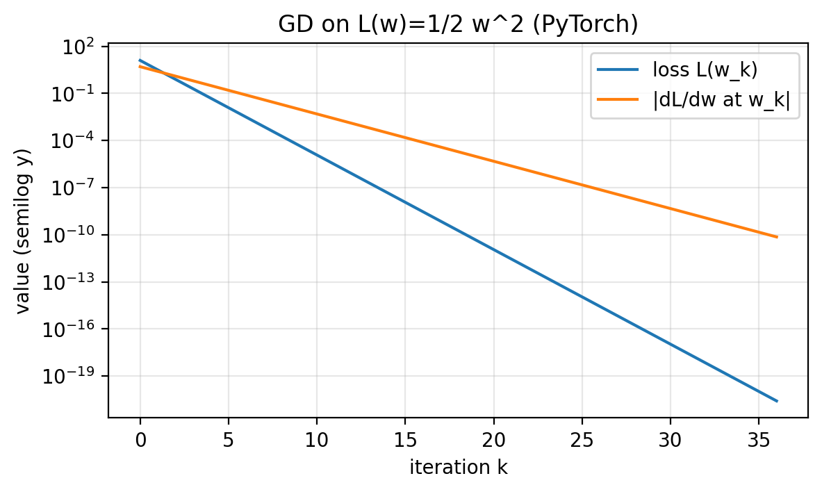 Figure 1.4: Same diagnostics as Figure 1.3, but derivatives are produced by autodiff.
8. Tuning: choosing a step size
The step size $\eta$ controls the tradeoff between:
- moving aggressively (fewer iterations when stable),
- not overshooting (avoiding divergence).
Quadratic example: exact recursion
Take
\[\begin{aligned} L(w) &= \tfrac{1}{2}w^2 \\ L'(w) &= w \end{aligned}\]Gradient descent gives:
\[w_{k+1}=w_k-\eta w_k = (1-\eta)w_k\]So:
- If $|1-\eta|<1$, then $w_k \to 0$ geometrically.
- If $|1-\eta|>1$, then $|w_k|$ grows geometrically (divergence).
For this specific quadratic, the stability condition is:
\[0 < \eta < 2\]A concrete divergence example: if $\eta=3$, then $w_{k+1}=-2w_k$, so $|w_k|$ doubles every step.
Compare small, reasonable, and too-large step sizes
We will compare:
- $\eta=0.001$ (stable but slow),
- $\eta=0.5$ (stable and fast),
- $\eta=3$ (diverges).
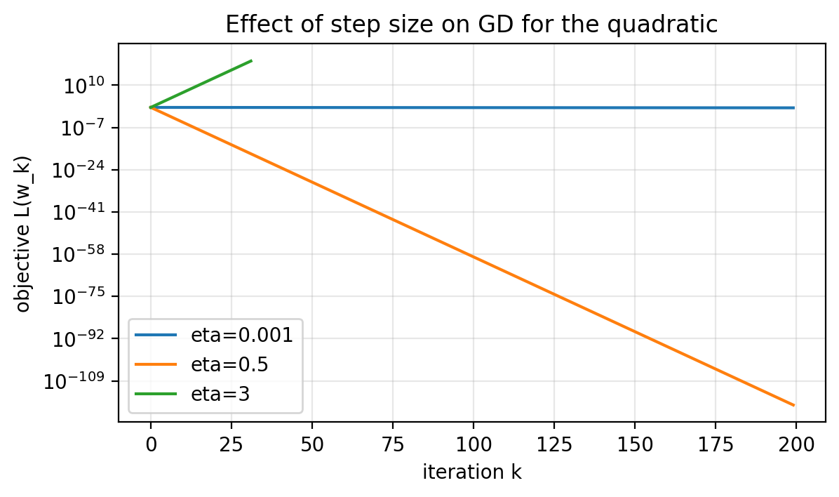 Figure 1.5: Same objective, same initialization, different step sizes. Small $\eta$ makes slow progress. Large $\eta$ diverges.
A simple tuning protocol: time-to-result
Fix a target:
\[L(w_k) \le 10^{-5}\]Define “time-to-result” as the number of iterations needed to hit this threshold (with a max-iteration cap).
For the quadratic, the recursion shows $\eta=1$ is special: it sends $w_1=0$ from any $w_0$.
You can still do the empirical version: sweep a range of step sizes and record the iteration count.
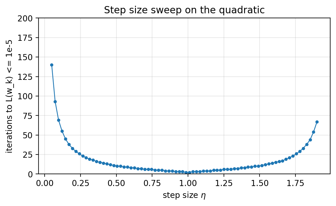 Figure 1.6: A brute-force sweep of step sizes. For this quadratic, the winner is near $\eta=1$.
Repeat on a nonconvex objective
For the double well,
\(L(w)=\tfrac{1}{2}(w^2-1)^2\) there are two global minimizers ($w=-1$ and $w=1$), and the curvature depends on where you are. A fixed step size can behave differently depending on initialization.
We can still run the same tuning sweep, but we must interpret it carefully: we are measuring “time-to-reach a minimizer” from a fixed starting point. To make the sweep informative, we start at $w_0=2$; for larger initializations the successful step-size range can shrink.
Here we sweep a wider range of step sizes; runs that do not reach the target within the cap show up at the max-iteration ceiling.
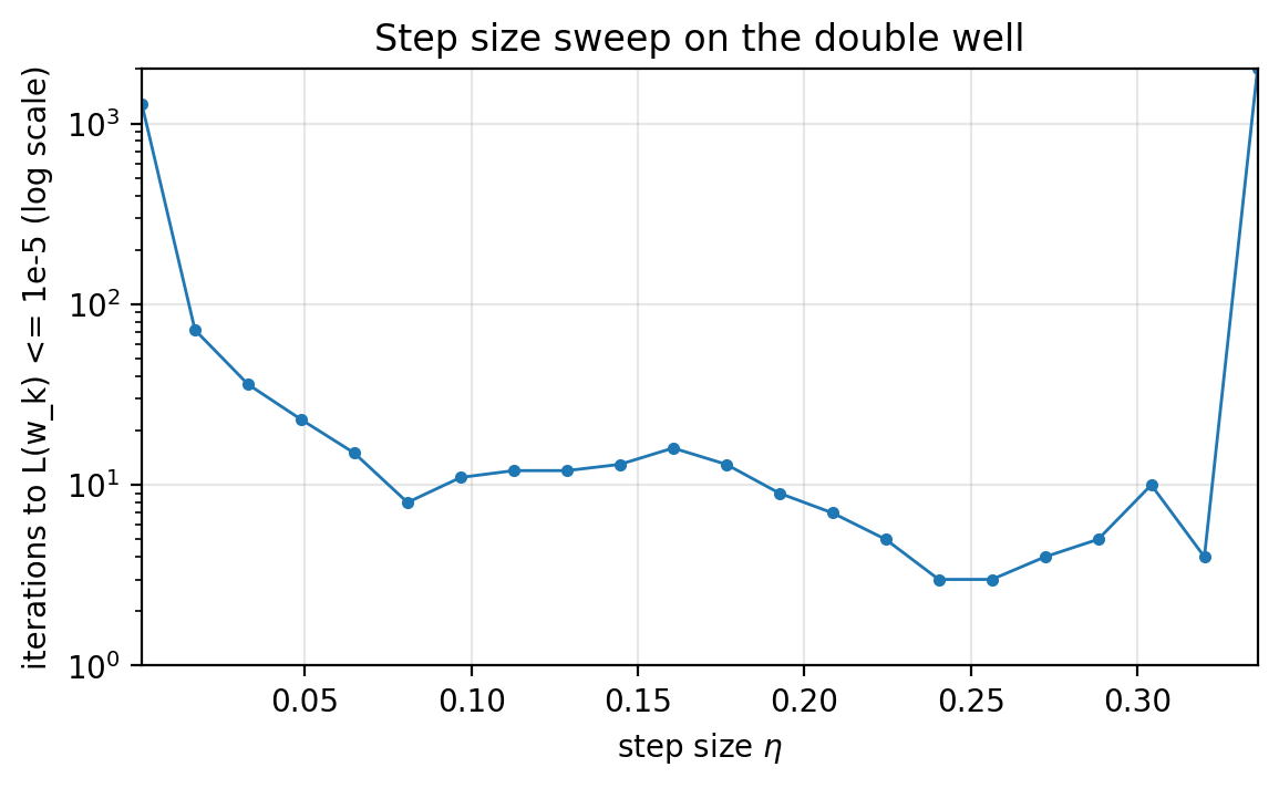 Figure 1.7: The best fixed step size depends on the objective and the initialization. For nonconvex problems, sweeping hyperparameters is often the pragmatic baseline.
9. Conclusion
What you should take from this lecture:
- An optimization problem is: decision variable + objective + constraints.
- Minimizers and stationary points are different targets. In nonconvex settings, stationarity is the default guarantee.
- Iterative algorithms should be judged by diagnostics and by time-to-result, not by whether they run.
- Gradient descent is a local method derived from the first-order Taylor model.
- With hand-written derivatives, changing the loss forces you to update derivative code too.
- With autodiff, you can change the loss without rewriting derivatives, as long as you follow a few PyTorch conventions:
- mark variables with
requires_grad=True, - clear
w.gradeach iteration, - update parameters under
torch.no_grad().
- mark variables with
Next lecture: we move from full gradients to stochastic gradient descent, where gradients are estimated from training samples.