Lecture 11 Cheat Sheet: A Playbook for Tuning Deep Learning Models

1. Introduction: Beyond Algorithms to Process

• Problem: Deep learning success relies heavily on the process of tuning, which is often undocumented and ad-hoc. (Ref: Playbook Intro [1])
• Goal: Present a systematic, evidence-based workflow for tuning, based on the Deep Learning Tuning Playbook [1] and empirical findings [2, 3].
• Context: Builds on Lectures 6-9 (algorithms) and Lecture 10 (comparison challenges). Focuses on how to tune effectively and reproducibly.

Overall Workflow Visualization:

Figure 1: Overview of the iterative tuning process based on the Deep Learning Tuning Playbook [1]. […] (See full caption in lecture notes)

2. Initial Setup: Foundational Choices

(Goal: Establish a simple, reasonable baseline before iterative tuning)

• Architecture (Sec 2.1):
  • Start with established, standard architectures for the task.
  • Defer custom architectures until later.
  • Architecture choice implies a family (hyperparameters like layers/width tuned later).
• Optimizer (Sec 2.2):
  • Start with popular, well-understood optimizers (SGD+Momentum, Adam, AdamW - See L7, L9).
  • Consider the tuning effort trade-off: More complex optimizers (e.g., Adam: $η, \beta_1, \beta_2, \epsilon$) require tuning more hyperparameters than simpler ones (e.g., SGD+Momentum: $η, \beta$). (Ref: Playbook [1], implicitly Choi et al. [2])
  • Option: Start simpler (e.g., Adam with fixed $\beta$s, $\epsilon$) if resources are limited initially.
• Batch Size (Sec 2.3):
  • Primary role: Governs training speed & hardware use.
  • NOT a hyperparameter for directly tuning validation performance. (Ref: Playbook [1], Shallue et al. [3])
  • Comparable validation accuracy achievable across batch sizes IF other HPs (LR, regularization) are re-tuned. (Ref: Shallue et al. [3])
  • Scaling Pattern: Steps vs. Batch Size shows: Perfect Scaling -> Diminishing Returns -> Maximal Parallelism. 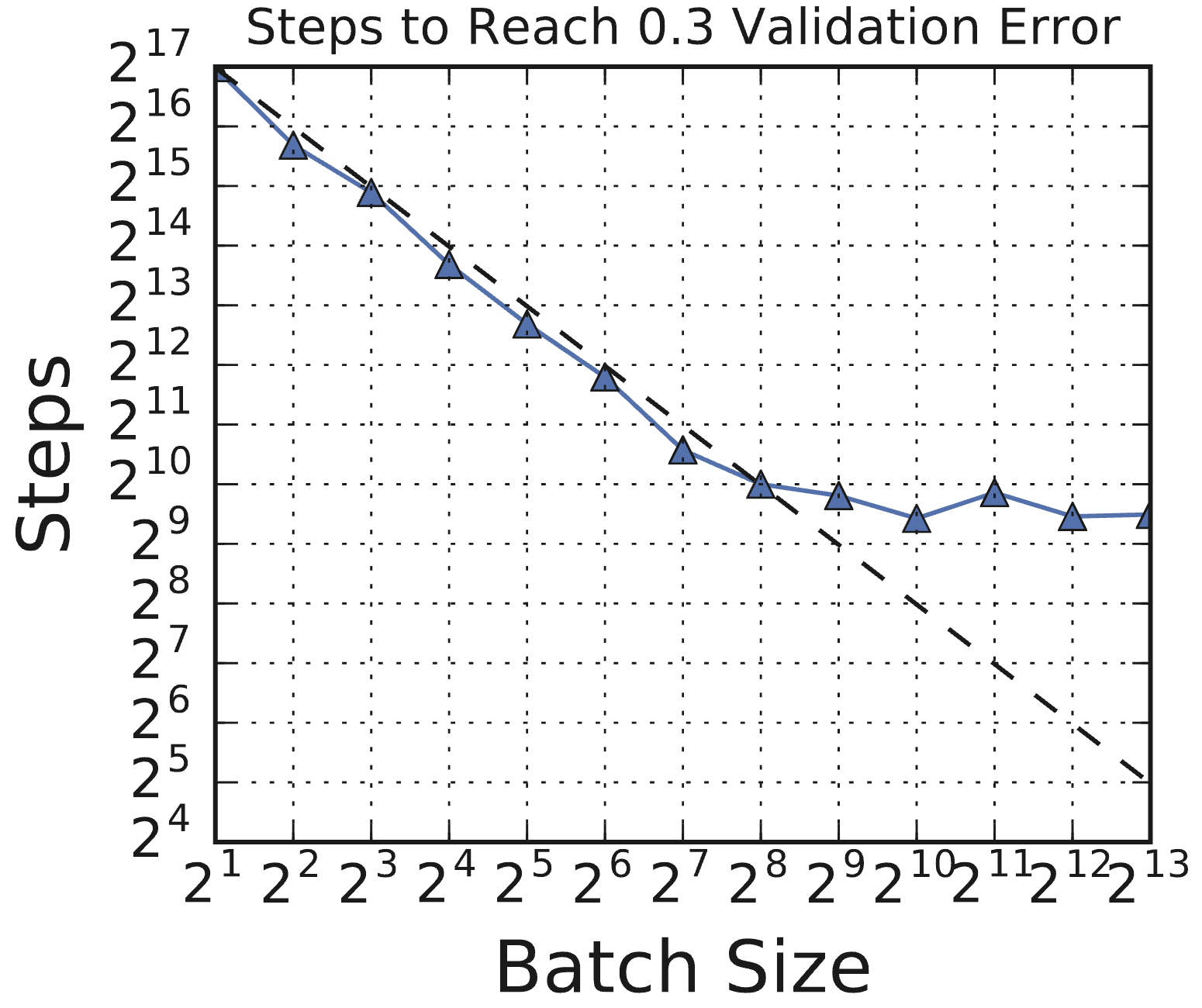(Source: Shallue et al., 2018, Fig 1c)
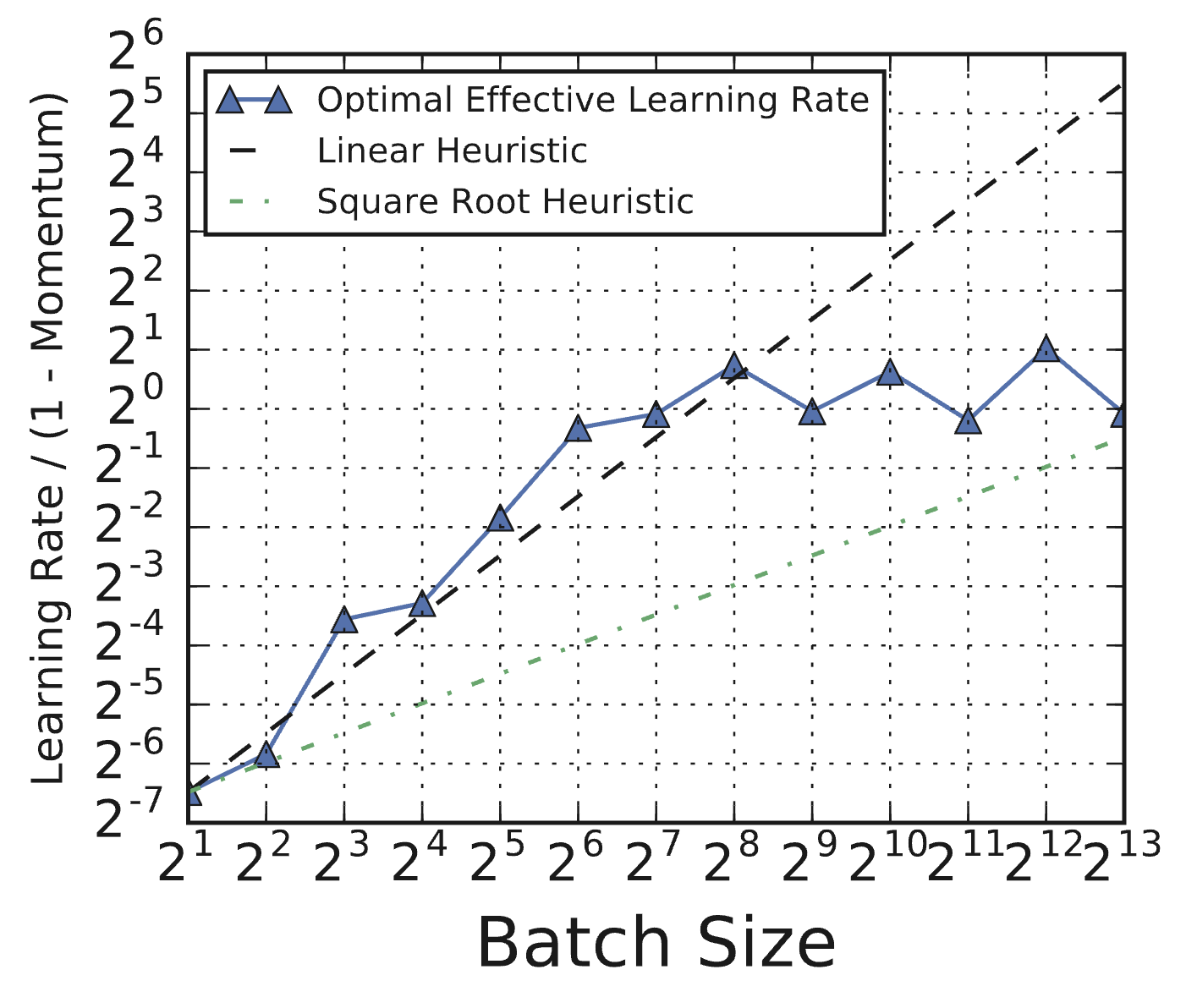
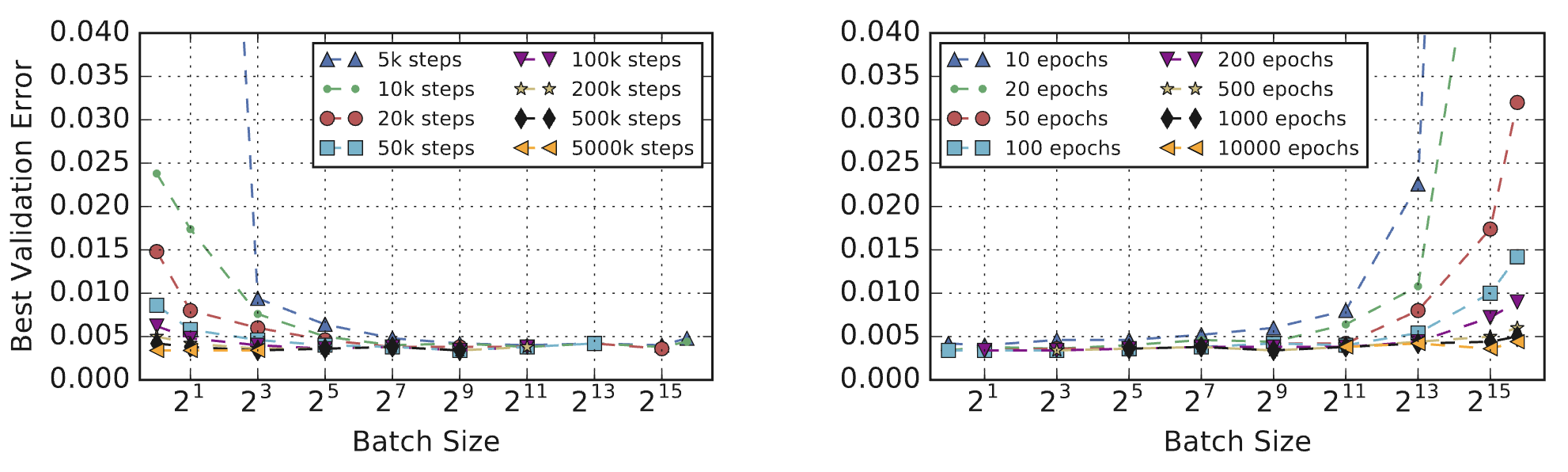
  • Re-tuning Need: Optimal LR often doesn’t follow simple scaling heuristics (linear/sqrt). Regularization needs may also change. (Source: Shallue et al., 2018, Fig 8c)
  • Epoch budgets vs. Step budgets yield different optimal batch sizes regarding validation error. Step budgets align better with minimizing wall-clock time. (Source: Shallue et al., 2018, Fig 11a)
• Initial Baseline (Sec 2.4):
  • Aim for: Simple, Resource-Efficient, Reasonable Performance (better than chance).
  • Start with minimal complexity (e.g., constant LR).
  • Initial training steps: Trade-off between faster iteration vs. easier schedule tuning (more in Sec 4).

3. The Tuning Process: Iterative & Scientific (Ref: Fig 1 Workflow)

(Goal: Improve performance incrementally via exploration and evidence-based decisions)

• Incremental Strategy (Sec 3.1):
  • Start simple (baseline).
  • Introduce changes one at a time.
  • Adopt changes (“launch” new baseline) only based on strong evidence of improvement.
  • Avoids unnecessary complexity.
• Exploration > Exploitation (Sec 3.2):
  • Focus: Most time spent on Exploration (gaining insight into the problem) not Exploitation (greedy optimization).
  • Benefits: Understand HP sensitivity/interactions, identify issues (overfitting), avoid spurious improvements, know when tuning saturates.
• Structuring Experiments (Sec 3.3):
  • Organize into “rounds” with a single, narrow goal.

  • Hyperparameter Roles (per round):

    - Scientific: Effect being investigated.
    - Nuisance:   Must be optimized over for fair comparison.
    - Fixed:      Held constant (introduces caveats).
    

  • Role depends on the goal (e.g., testing weight decay: presence=scientific, strength $λ$=nuisance).
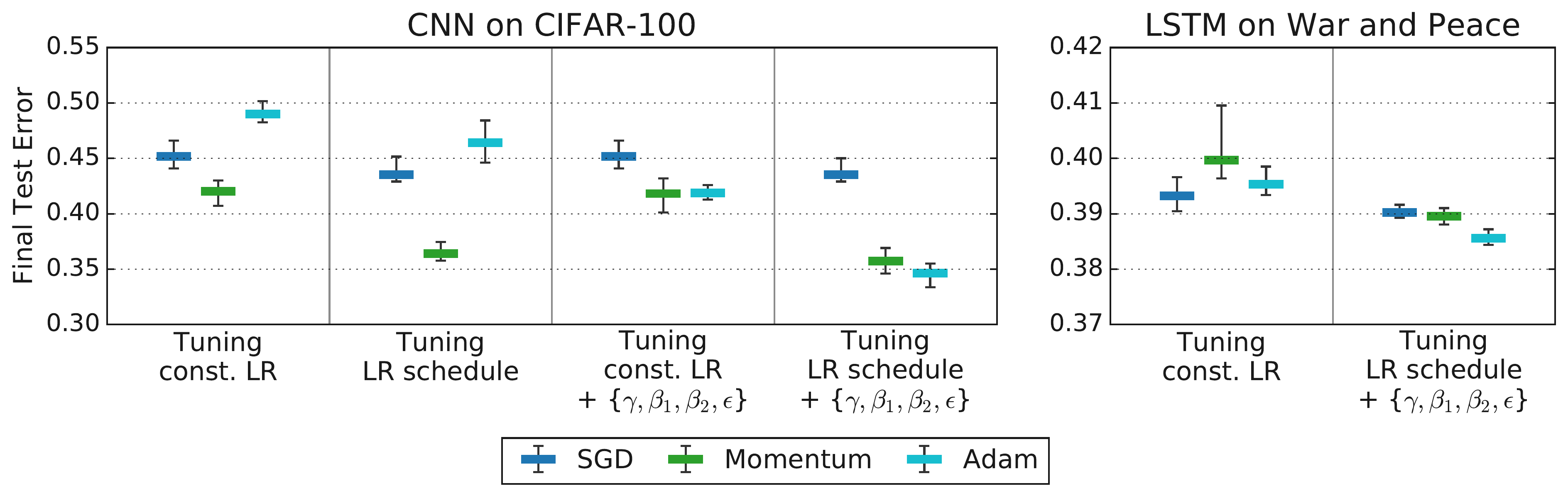
  • Critical Importance of Tuning Nuisance HPs: Fair comparison requires optimizing interacting nuisance HPs (like LR) for each setting of the scientific HP. Insufficient tuning leads to unreliable conclusions. (Ref: Choi et al. [2]) (Source: Choi et al., 2019b, Fig 3)
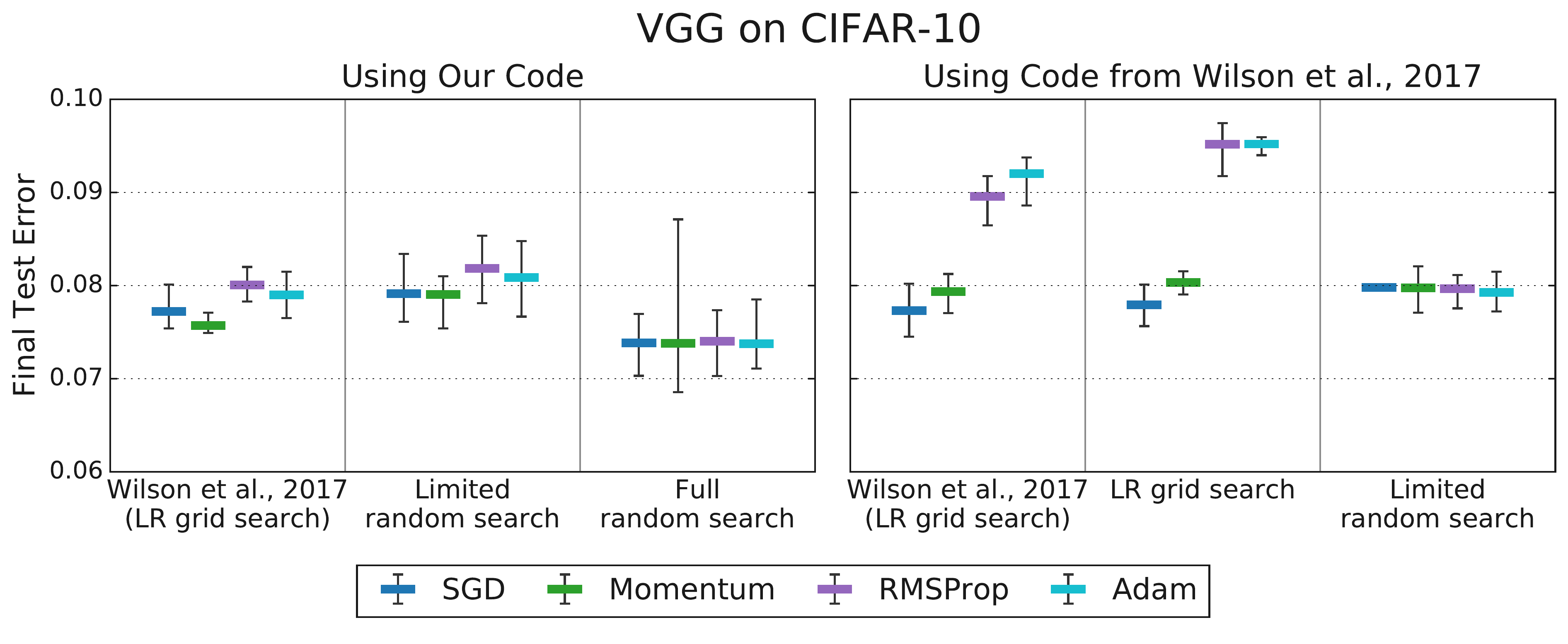
  • Tuning Protocol is Part of the Algorithm: Optimizer rankings depend heavily on the search space, budget, and method used for tuning. Comparisons are only valid if the protocol is defined and consistent. (Ref: Choi et al. [2]) (Source: Choi et al., 2019b, Fig 4)
  • Trade-offs: Balancing resources vs. caveats when deciding nuisance vs. fixed HPs. Optimizer HPs often nuisance; Arch HPs often scientific/fixed.
  • Conditional HPs: Some HPs only exist for certain scientific HP values (e.g., Adam’s βs).
• Designing Studies (Sec 3.4):
  • Study = set of trials (configurations).
  • Goal: Compare scientific HPs by optimizing over nuisance HPs.
  • Search Method:
    • Exploration Phase: Use Quasi-Random Search (non-adaptive, uniform coverage, good for parallelism/analysis). (Ref: Playbook [1], Bousquet et al. [4])
    • Exploitation Phase: Use Bayesian Optimization (adaptive, focuses search). (Ref: Playbook [1], Gelbart et al. [5])
  • Budget Allocation: Balance # scientific values vs. nuisance space size vs. sampling density.
• Analyzing Results (Sec 3.5):
  • Go beyond the primary goal; look for insights & issues.
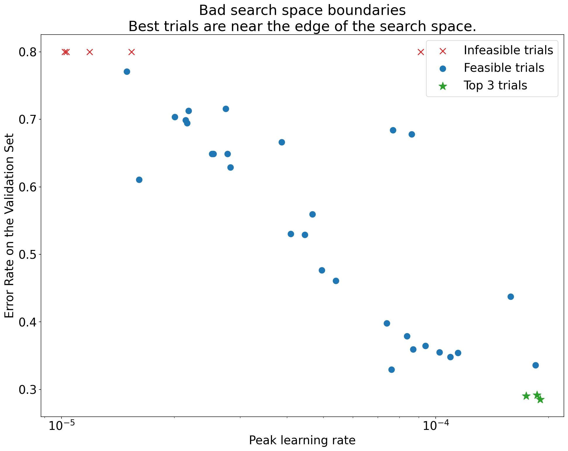
  • Check Search Boundaries: Use axis plots (Perf vs. HP). Best trials near edge? -> Expand space. 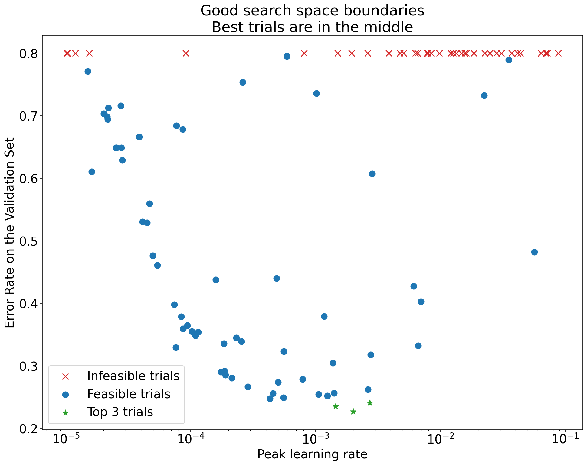(Caption: See Lecture Notes Figure 6)
  • Check Sampling Density: Is the “good” region well-covered? (Hard to quantify, use plots).
  • Examine Training/Validation Curves (Best Trials):
    • Problematic Overfitting? (Val loss increases) -> Need more regularization.
    • High Variance? (Noisy curves) -> Affects comparison; consider ↑BS, LR decay, Polyak avg.
    • Still Improving? -> Maybe need more steps (Sec 4).
    • Saturated Early? -> Maybe too many steps (Sec 4).
  • Use Isolation Plots: Compare scientific HPs after optimizing nuisance HPs. 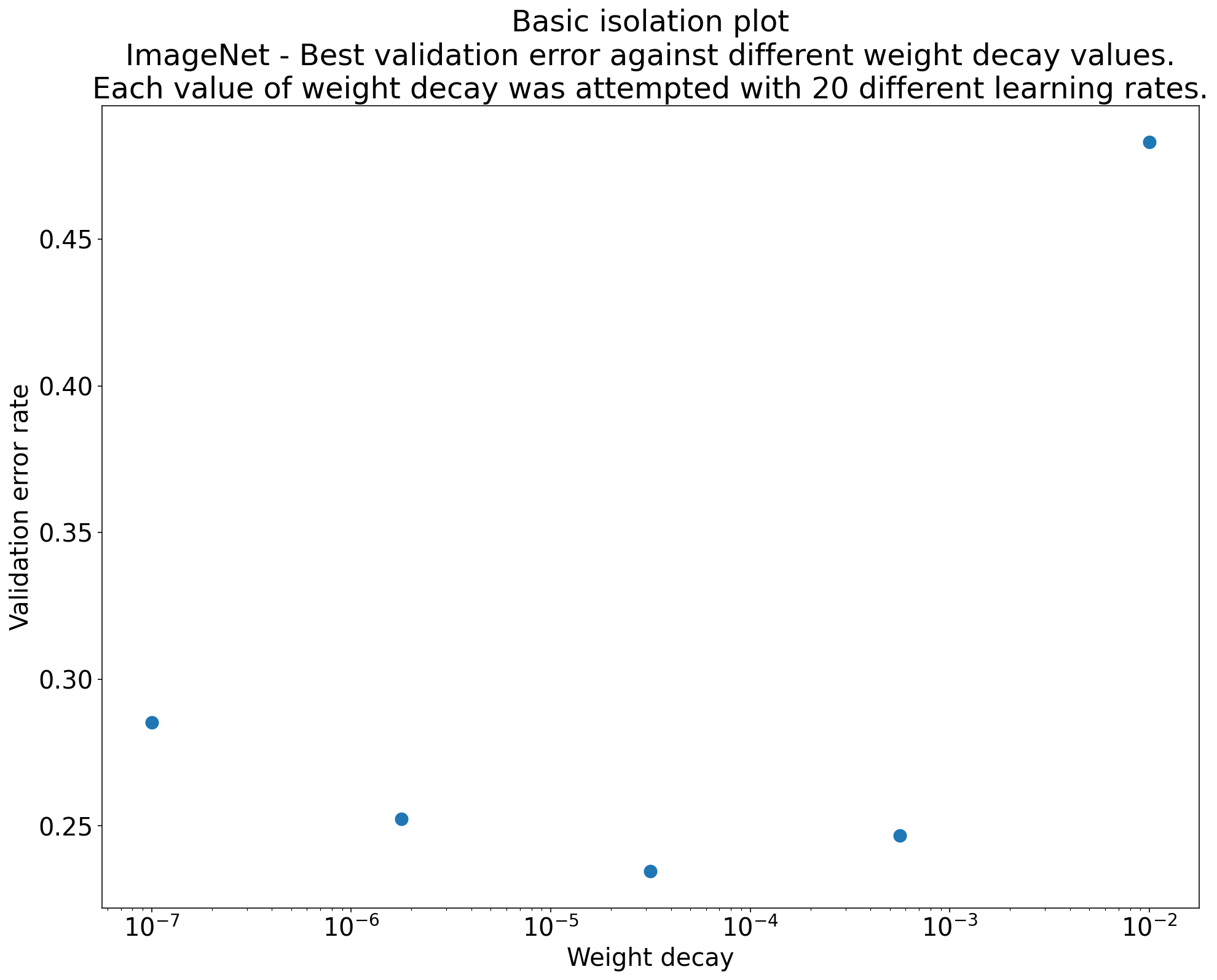(Caption: See Lecture Notes Figure 7)
• Making Decisions (Sec 3.6):
  • Adopt change if improvement > variance (trial & study) and worth added complexity.
  • Characterize trial variance by rerunning best trials if feasible.

4. Determining Training Duration

• Regimes: Compute-bound (longer helps) vs. Not compute-bound (performance saturates).
• Protocol:
  • Use a fixed max_train_steps for all trials within a study.
  • Do NOT tune max_train_steps as a hyperparameter within the study.
  • Use retrospective checkpoint selection (save best checkpoint based on validation performance during the run).
  • Observe where best checkpoints land to inform max_train_steps for future rounds.
  • Interacts strongly with LR decay schedule tuning.

5. Conclusion

• Effective tuning is a systematic, iterative, scientific process, not random tweaking. (Ref: Playbook [1])
• Focus on exploration & insight for most of the process.
• The tuning protocol IS part of the algorithm for empirical comparisons. Fair comparisons require tuning nuisance HPs. (Ref: Choi et al. [2])
• Adopt changes based on evidence, considering variance and complexity.