Slide 1: Scaling Transformers: Parallelism Strategies from the Ultrascale Playbook

(Based on Hugging Face Ultrascale Playbook)

Goal: Understand why and how we train massive AI models across many computers.

Slide 2: The Scaling Challenge

Why are we here?

• Modern AI models (like Transformers) are HUGE (Billions/Trillions of parameters!).
• Too big for one computer (specifically, one GPU’s memory).
• Need to split the work across many GPUs/computers.

Today’s Focus:

• System-level challenges & strategies for distributed training.
• How to manage computation & memory across devices.
• (Not focusing on the optimization math itself).

Core Resource: Hugging Face Ultrascale Playbook (link)

Slide 3: What IS a Transformer? (The Big Picture)

Purpose: Process sequences (like text) and understand relationships between elements (words).

Core Idea: Input sequence -> Embeddings -> Many Transformer Blocks -> Output Layer

(A simple block diagram showing Input -> Embedding -> L x Blocks -> Output)

Key: The “Transformer Block” is where most complexity and computation happens. We stack many ($L$) of these blocks.

Slide 4: Transformer Anatomy 1: Input & Embedding

Input: Sequence of tokens (integer IDs): $x = (x_1, \dots, x_s)$ (length $s$)

1. Embedding Layer:

• Map each token ID $x_i$ to a vector.
• Uses a learnable matrix $W_E \in \mathbb{R}^{V_{size} \times h}$.
  • $V_{size}$: Vocabulary size (how many unique words/tokens)
  • $h$: Hidden dimension (size of the vector for each token)
• Result: $H^{(0)}_{\text{embed}} \in \mathbb{R}^{s \times h}$ (a sequence of vectors)

2. Positional Encoding:

• Transformers don’t inherently know word order. Add position info!
• Uses fixed or learned vectors $P \in \mathbb{R}^{s \times h}$.
• Resulting initial representation: $H^{(0)} = \text{Embed}(x) + P \in \mathbb{R}^{s \times h}$

Parameters here: Mostly $W_E$ (can be large if $V_{size}$ is big).

Slide 5: Transformer Anatomy 2: Layer Normalization (LN)

Purpose: Stabilizes training, helps gradients flow. Applied before main sub-layers (Pre-LN).

What it does: Normalizes features across the hidden dimension ($h$) for each token independently.

Input: Tensor $Z \in \mathbb{R}^{s \times h}$ (e.g., $H^{(l-1)}$) Output: Normalized Tensor $\text{LN}(Z) \in \mathbb{R}^{s \times h}$

Formula (for token $i$): \(\text{LN}(Z)_i = \gamma \odot \frac{Z_i - \mu_i}{\sqrt{\sigma_i^2 + \epsilon}} + \beta\)

• $\mu_i, \sigma_i^2$: Mean/Variance across hidden dim $h$ for token $i$.
• $\gamma, \beta \in \mathbb{R}^h$: Learnable scale & shift parameters (element-wise $\odot$).
• $\epsilon$: Small constant for stability.

Parameters per LN layer: $2h$ (from $\gamma, \beta$). Used multiple times in each block!

Slide 6: Transformer Anatomy 3: The Transformer Block

Core Unit: Repeated $L$ times. Input $H^{(l-1)}$, Output $H^{(l)}$. Two Main Sub-Layers:

1. Multi-Head Self-Attention (MHA)
2. Position-wise Feedforward Network (FFN)

Structure (Pre-LN Variant):

Input H^(l-1) --> LN1 --> MHA --> Add (*) --> LN2 --> FFN --> Add (**) --> Output H^(l)
                  |         |                 |         |
                  +---------+ (Residual 1)    +---------+ (Residual 2)

• LN1, LN2: Layer Normalization.
• Add (*, **): Residual Connections (add input to output of sub-layer). Crucial for depth!

Slide 7: Transformer Anatomy 4: Multi-Head Attention (MHA) - Part 1

Purpose: Allows each token to look at other tokens in the sequence and decide which are important (“attend to”).

Input: Normalized $ X’ = \text{LN}_1(H^{(l-1)}) $

1. Create Query, Key, Value vectors:

• Linearly project $X’$ using learnable weights $W_Q, W_K, W_V \in \mathbb{R}^{h \times h}$. \(Q = X' W_Q, \quad K = X' W_K, \quad Val = X' W_V\)
  • $Q$: What I’m looking for.
  • $K$: What I contain.
  • $Val$: What I’ll give you if you attend to me.

2. Split into Multiple Heads:

• Divide $Q, K, Val$ (dim $h$) into $a$ smaller chunks (“heads”) along the hidden dim.
• $Q_i, K_i, Val_i \in \mathbb{R}^{s \times d_k}$ where $d_k = h/a$.
• Why heads? Allows model to focus on different types of relationships simultaneously.

Parameters: $W_Q, W_K, W_V$ (total $3h^2$).

Slide 8: Transformer Anatomy 5: Multi-Head Attention (MHA) - Part 2

3. Scaled Dot-Product Attention (per head $i$):

• Calculate attention scores: How much should query $q$ attend to key $k$? \(\text{RawScores}_i = Q_i K_i^T \in \mathbb{R}^{s \times s}\)
• Scale scores (stabilizes gradients): Divide by $\sqrt{d_k}$.
• Normalize scores (sum to 1 per query): Apply Softmax row-wise. \(\text{Scores}_i = \text{softmax}_{\text{keys}}\left(\frac{Q_i K_i^T}{\sqrt{d_k}}\right) \in \mathbb{R}^{s \times s}\)

4. Get Weighted Values:

• Multiply scores by Value vectors: \(O_i = \text{Scores}_i \cdot Val_i \in \mathbb{R}^{s \times d_k}\)
  • Output is weighted sum of values, based on attention scores.

Computation: Matrix Multiplies ($QK^T$, $\text{Scores} \cdot Val$) are dominant. $QK^T$ scales with $s^2$!

Slide 9: Transformer Anatomy 6: Multi-Head Attention (MHA) - Part 3

5. Concatenate Heads:

• Combine outputs from all heads back together: \(O_{concat} = \text{Concat}(O_1, \dots, O_a) \in \mathbb{R}^{s \times h}\)

6. Final Output Projection:

• Apply one more linear layer $W_O \in \mathbb{R}^{h \times h}$: \(O_{MHA} = O_{concat} W_O\)

7. Add Residual:

• $H_{intermediate} = H^{(l-1)} + O_{MHA}$ (Connect back to block input)

Parameters: $W_O$ ($h^2$). Total MHA params: $4h^2$ (ignoring biases). Key Computations: Projections (Q, K, V, O), Attention ($QK^T$, Score*V).

Slide 10: Transformer Anatomy 7: Feedforward Network (FFN)

Purpose: Process information for each token independently after attention. Adds representational capacity.

Input: Normalized $ X’’ = \text{LN}_2(H_{intermediate})$

Structure: Two linear layers with a non-linearity (e.g.,GELU) in between. \(O_{FFN} = \text{GELU}(X'' W_1 + b_1) W_2 + b_2\)

• $W_1 \in \mathbb{R}^{h \times d_{ff}}$, $b_1 \in \mathbb{R}^{d_{ff}}$ (Expand dimension)
• $W_2 \in \mathbb{R}^{d_{ff} \times h}$, $b_2 \in \mathbb{R}^{h}$ (Contract back to $h$)
• $d_{ff}$ is the intermediate “feedforward dimension”, often $d_{ff}=4h$.

Add Residual:

• $H^{(l)} = H_{intermediate} + O_{FFN}$ (Output of the block)

Parameters: $W_1, b_1, W_2, b_2$ (Roughly $2 \times h \times d_{ff} \approx 8h^2$ params). Computation: Dominated by two large matrix multiplies.

Slide 11: Transformer Anatomy 8: Final Layers, Loss, & Summary

After Last Block ($L$):

• Optional Final LayerNorm: $H’_{final} = \text{LN}_{final}(H^{(L)})$
• Output Layer: Project to final task output (e.g., vocabulary logits for language modeling).
  • Uses $W_{LM} \in \mathbb{R}^{h \times V_{size}}$ (often tied/shared with $W_E$).
  • $ \text{Logits} = H’_{final} W_{LM} \in \mathbb{R}^{s \times V_{size}}$
  • Each row $\text{Logits}_i \in \mathbb{R}^{V_{size}}$ contains scores for each possible next token at position $i$.

Calculating the Loss (How the model learns):

• Purpose: Quantify how wrong the model’s predictions are compared to the actual target sequence.
• Input:
  • Model $\text{Logits} \in \mathbb{R}^{s \times V_{size}}$.
  • Target sequence (true next tokens): $y = (y_1, \dots, y_s)$, where $y_i$ is the integer index of the correct token at position $i$.
• Common Loss Function (Language Modeling): Cross-Entropy Loss
  • Compares the predicted probability distribution (derived from logits via Softmax) with the target (which is 1 for the correct token, 0 otherwise).
  • Formula (average over sequence): \(\ell(W) = -\frac{1}{s} \sum_{i=1}^s \log \left( \frac{\exp(\text{Logits}_{i, y_i})}{\sum_{j=1}^{V_{size}} \exp(\text{Logits}_{i, j})} \right)\)
    • Essentially: Maximize the log-probability of the correct next token $y_i$ at each position $i$.
• Goal of Training: Find model parameters $W = {W_E, W_Q, …, W_{LM}}$ that minimize this loss $\ell(W)$. Backpropagation calculates $\nabla_W \ell$.

Parameter Summary (Same as before):

• Embeddings: $W_E$ ($V_{size}h$)
• MHA Layers (per block): $W_Q, W_K, W_V, W_O$ ($4h^2$)
• FFN Layers (per block): $W_1, W_2$ (~$8h^2$)
• LayerNorms (per LN): $\gamma, \beta$ ($2h$)
• Output Projection: $W_{LM}$ ($h V_{size}$)
• Total: Scales roughly as $O(V_{size}h + Lh^2)$.

Computation Summary (Same as before):

• Matrix Multiplies in MHA ($QK^T$, Score*V)
• Matrix Multiplies in FFN ($XW_1$, $HW_2$)
• Repeated $L$ times! + Final Projection + Loss Calc.

Slide 12: Transformer Anatomy 9: Common Modifications

1. Attention Masking:

• Purpose: Control which tokens can attend to which others.
• How: Add large negative values ($-\infty$) to attention scores before softmax. \(\text{Scores}_i = \text{softmax}_{\text{keys}}\left(\frac{Q_i K_i^T}{\sqrt{d_k}} + M\right)\)
• Example: Causal Mask (for Autoregressive LM): Prevent attending to future tokens ($M_{jk} = -\infty$ if $k > j$).
• Doesn’t add parameters, changes computation slightly.

2. Dropout:

• Purpose: Regularization during training (prevent overfitting).
• How: Randomly set some activation values to 0, scale the rest.
• Applied after MHA output, within FFN, etc.
• Deactivated during inference (testing).
• Adds one hyperparameter (dropout rate $p$).

Slide 13: The Memory Bottleneck: Activations!

Problem: Training needs gradients ($\nabla_w \ell$). Backpropagation computes them using the chain rule.

Key Requirement: Backprop needs intermediate values (“activations”) computed during the forward pass.

Example: To compute $\nabla_W$ for $Y=XW$, we need $X$. To compute $\nabla_X$, we might need $Y$ or internal values.

Consequence: We must store many intermediate tensors ($Q, K, V$, attention scores, FFN hidden states, layer outputs $H^{(l)}$, etc.) until they’re used in the backward pass.

This takes a LOT of memory!

Slide 14: Activation Memory vs. Parameter Memory

Activation Memory:

• Stores intermediate results from forward pass.
• Depends on:
  • Batch Size (b)
  • Sequence Length (s)
  • Hidden Dimension (h)
  • Number of Layers (L)
• Scales Roughly: $O(L \times b \times s \times h)$ (plus terms like $b \times a \times s \times s$ for attention scores!)
• Grows with batch size b and sequence length s!

Parameter Memory:

• Stores model weights ($W_E, W_Q, …$).
• Depends on: $V_{size}, h, L, d_{ff}$.
• Scales Roughly: $O(V_{size}h + Lh^2)$.
• Independent of batch size b and sequence length s!

The Bottleneck: For large models/batches/sequences, Activation Memory » Parameter Memory. This limits what fits on a single GPU.

Slide 15: Solution 1: Activation Recomputation (Gradient Checkpointing)

Idea: Trade compute time for memory savings.

How:

1. Forward Pass: Compute as usual, but don’t store all intermediate activations. Store only a few strategic ones (e.g., inputs to major blocks $H^{(l-1)}$).
2. Backward Pass: When a needed activation wasn’t stored, recompute it on the fly by running a small part of the forward pass again, starting from the nearest stored activation.

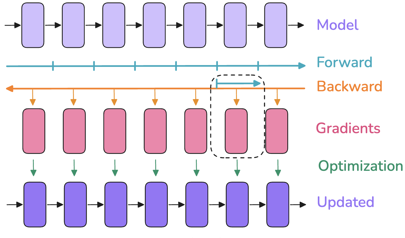(Top: Standard backprop stores everything. Bottom: Recomputation stores less, recomputes needed values during backward pass.)

Trade-off:

• Pro: Significantly reduces activation memory footprint.
• Con: Increases computation time (roughly adds one extra forward pass for recomputed segments).
• Often essential for training very large models.

Reference: Playbook Section

Slide 16: Toolbox: Distributed Communication Primitives (Why?)

Problem: We need multiple GPUs (workers) to cooperate. They need to exchange data.

Solution: Use standard communication patterns (“collectives”).

Context:

• Group of $N$ workers, each with a rank (0 to $N-1$).
• Usually implemented by libraries like NCCL for high-speed GPU communication.

Understanding these is key to understanding parallelism strategies!

Reference: Playbook Appendix A0

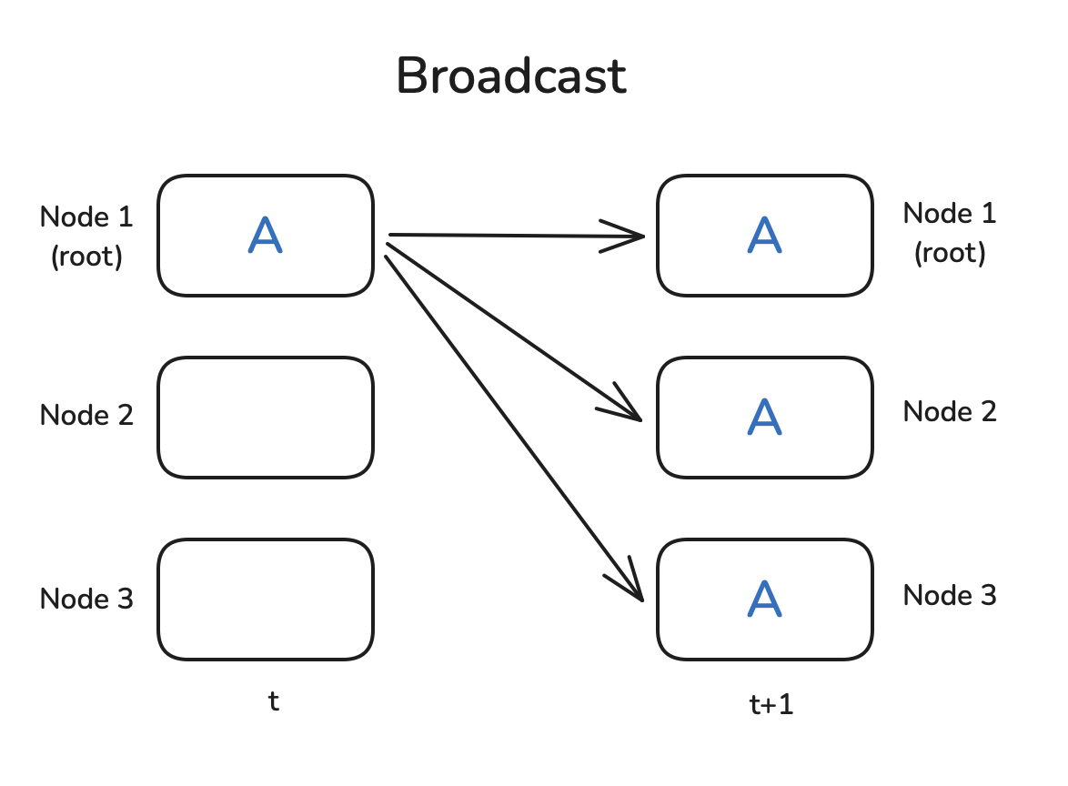
Slide 17: Primitives 1: Broadcast & Reduce/AllReduce

Broadcast: One worker sends the same data to all others (including itself).

• Use case: Send initial weights from rank 0 to all.

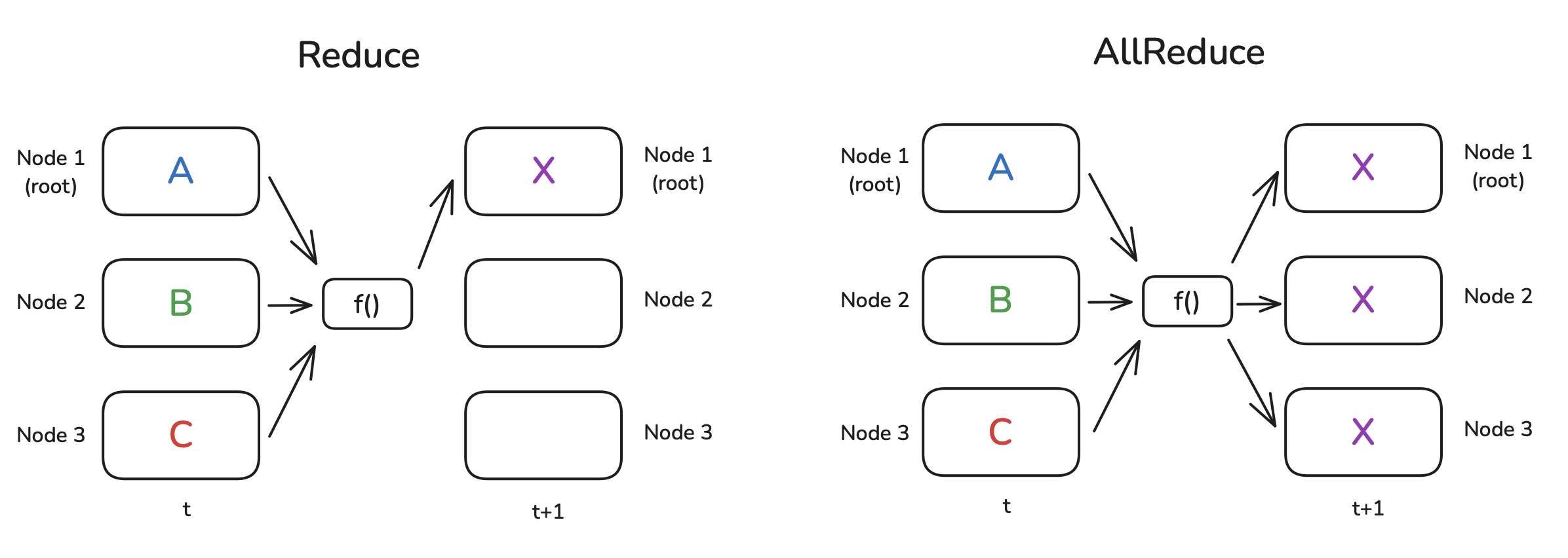
Reduce: Collect data from all workers, apply an operation (SUM, AVG), store result on one destination worker.

• Use case: Aggregate partial results onto one worker.

AllReduce: Like Reduce, but the final result is distributed back to all workers.

• Use case: Average gradients across all workers in Data Parallelism.

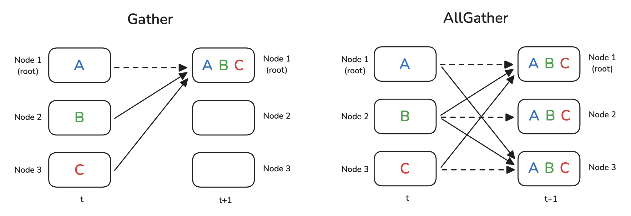
Slide 18: Primitives 2: Gather/AllGather & Scatter/ReduceScatter

Gather: Collect different data chunks from each worker onto one destination worker.

• Use case: Collect results from different workers.

AllGather: Like Gather, but the collected result (all chunks) is distributed back to all workers.

• Use case: Reconstruct a full tensor from shards held by different workers (ZeRO).

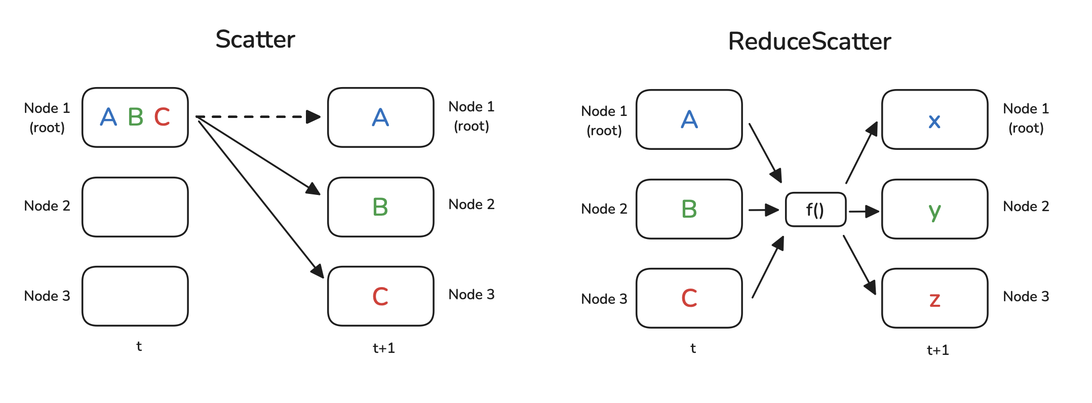
Scatter: One source worker sends different chunks of data to each worker. (Inverse of Gather).

• Use case: Distribute parts of a dataset.

ReduceScatter: Combine Reduce and Scatter. Reduce corresponding chunks from all workers, then Scatter the reduced chunk $j$ only to worker $j$.

• Use case: Compute and distribute sharded average gradients (ZeRO).

Slide 19: Primitives 3: Barrier & AlltoAll (Mentioned Later)

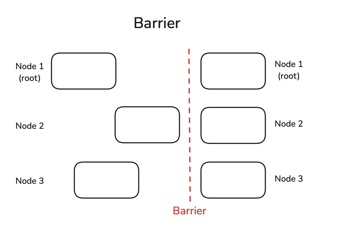
Barrier: Synchronization point. All workers wait here until everyone arrives.

• Use case: Ensure a stage is complete everywhere before proceeding. (Use sparingly - can cause waiting).

(Preview) AlltoAll: Each worker sends different data to every other worker. Worker $i$ sends chunk $j$ to worker $j$. Complex permutation.

• Use case: Routing tokens to specific “expert” networks in MoE models (Expert Parallelism).

A helpful visualization

Visualization for DP, FSDP, and TP

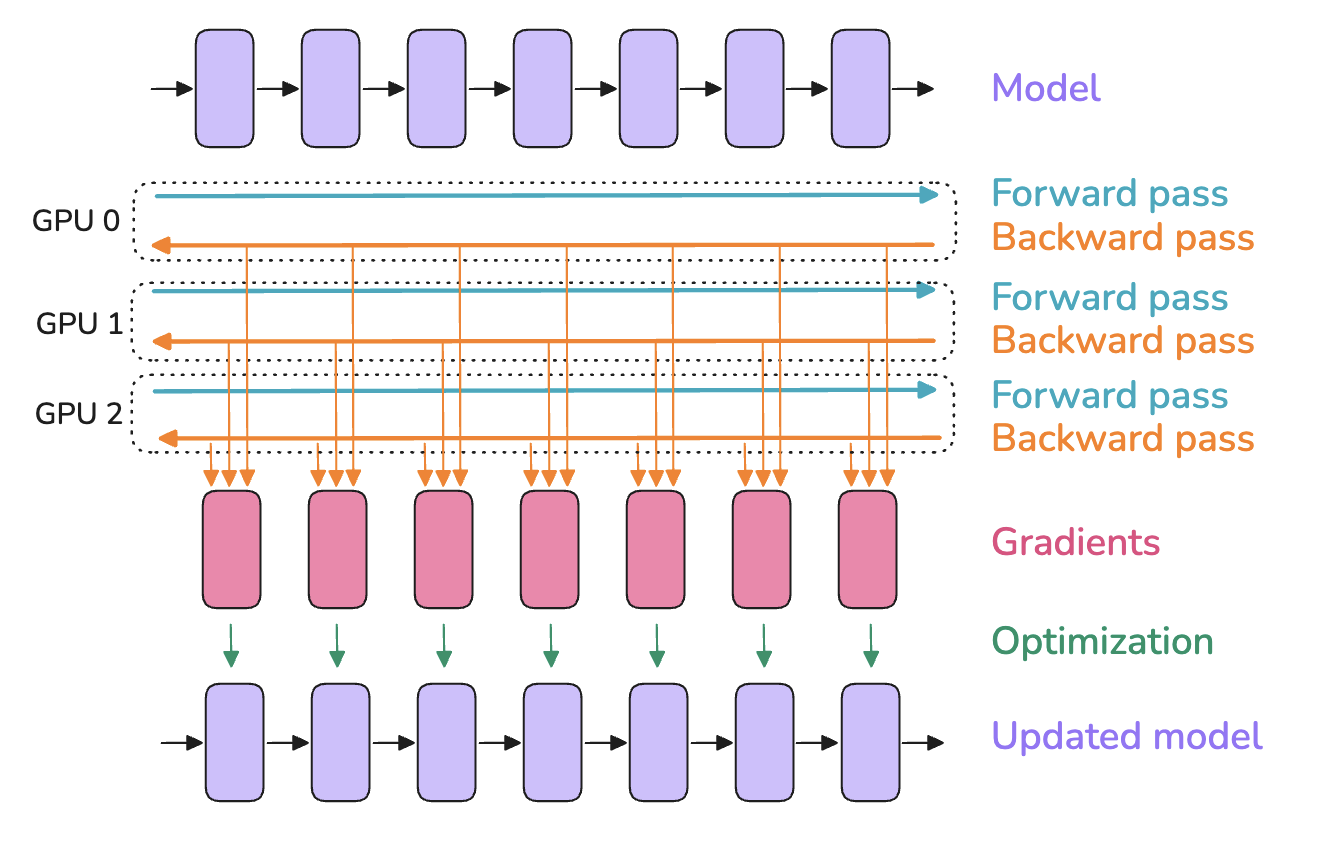
Slide 20: Parallelism Strategy 1: Data Parallelism (DP)

What: Replicate the entire model on each of $N_d$ workers. Split the data batch across workers. Why: Increase training throughput by processing more data in parallel. Simplest parallel strategy.

How:

1. Each worker $k$ gets a micro-batch $\mathcal{B}_k$.
2. Forward pass on $\mathcal{B}_k$ using local model $w \rightarrow$ Compute loss.
3. Backward pass $\rightarrow$ Compute local gradient $g_k$.
4. Synchronize Gradients: Average gradients across all workers: $\hat{g} = \frac{1}{N_d} \sum_k g_k$. Use AllReduce.
5. Each worker updates its local model copy using the same average gradient $\hat{g}$. $w_{t+1} = \text{OptimizerStep}(w_t, \hat{g})$.

Reference: Playbook Section

Slide 21: DP Optimizations: Overlap & Bucketing

Problem: Waiting for AllReduce is slow. Communication cost scales with model size $|w|$.

Solution 1: Overlap Communication & Computation:

• Start AllReduce for gradients of later layers while backward pass computes gradients for earlier layers.

Solution 2: Gradient Bucketing:

• Group gradients into larger “buckets”.
• Perform one AllReduce per bucket instead of per tensor.
• Reduces communication call overhead, improves bandwidth use, enables better overlap.

Slide 22: DP Concept: Gradient Accumulation

Purpose: Simulate a larger effective batch size without increasing memory per worker.

How:

1. Divide worker’s data $\mathcal{B}_k$ into $A$ smaller “accumulation micro-batches” $\mathcal{B}_{k,a}$.
2. For $a = 1$ to $A$:
   • Forward/Backward on $\mathcal{B}_{k,a}$ to get gradient $g_{k,a}$.
   • Accumulate gradients locally: $g_{k}^{(A)} = \sum_{a=1}^A g_{k,a}$.
   • Crucially: NO gradient synchronization (AllReduce) for steps $a=1..A-1$. (Use framework tools like no_sync()).
3. After step A: Perform one AllReduce on the accumulated gradients $g_{k}^{(A)}$.
4. Perform one optimizer step using the final averaged gradient.

Trade-off: Saves memory, but takes $A$ times longer computationally for the same amount of data compared to a single large batch.

Slide 23: DP Limitations

The Big Problem: Memory Redundancy!

• Every worker stores:
  • Full Model Parameters ($w$)
  • Full Optimizer States ($\text{OptState}$ - e.g., Adam moments, often 2x parameter size!)
  • Full Gradients ($g_k$) (at least temporarily)
  • Activations ($A_k$) for its micro-batch.
• Memory usage per worker does not decrease as you add more workers ($N_d$).
• DP alone cannot train a model that doesn’t fit on a single GPU.

Communication Bottleneck: AllReduce cost scales with model size $|w|$ and can limit scaling as $N_d$ increases.

Slide 24: Parallelism Strategy 2: ZeRO (Zero Redundancy Optimizer)

What: Enhance Data Parallelism by partitioning (sharding) model state (Optimizer States, Gradients, Parameters) across DP workers ($N_d$). Eliminates memory redundancy. Why: Train much larger models under DP by reducing memory per worker.

Core Idea: Worker $k$ only owns and updates shard $(k)$ of the state.

Reference: Playbook Section

Slide 25: ZeRO Stage 1 (ZeRO-1): Partition Optimizer States

• Partitions: Optimizer States ($\text{OptState}^{(k)}$).
• Replicates: Parameters ($w$), Gradients ($g_k$).

How:

1. Fwd/Bwd: Compute full local gradient $g_k$.
2. Sync/Shard Gradients: ReduceScatter sums gradients and gives worker $k$ only its needed shard $\hat{g}^{(k)}$.
3. Optimizer Step: Worker $k$ updates only its parameter shard $w^{(k)}$ using $\hat{g}^{(k)}$ and local $\text{OptState}^{(k)}$.
4. Sync Parameters: AllGather collects updated $w^{(k)}$ from all workers to reconstruct the full $w$ on every worker for the next step.

Memory Saved: Optimizer states (often the largest part!). Communication: Replaces 1 AllReduce with ReduceScatter + AllGather. Reference: Playbook Section

Slide 26: ZeRO Stage 2 (ZeRO-2): Partition Gradients Too

• Partitions: Optimizer States ($\text{OptState}^{(k)}$), Gradients ($\hat{g}^{(k)}$).
• Replicates: Parameters ($w$) (temporarily during compute).

How:

1. Fwd: Compute activations $A_k$.
2. Bwd & Shard Gradients: As gradients are computed, ReduceScatter them immediately. Worker $k$ only stores the final, averaged shard $\hat{g}^{(k)}$. (Avoids storing full $g_k$).
3. Optimizer Step: Update $w^{(k)}$ using $\hat{g}^{(k)}$ and $\text{OptState}^{(k)}$.
4. Sync Parameters: AllGather reconstructs full $w$.

Memory Saved: Optimizer states + Gradients. Communication: Still ReduceScatter + AllGather. Reference: Playbook Section

Slide 27: ZeRO Stage 3 (ZeRO-3 / FSDP): Partition Parameters Too

• Partitions: Optimizer States ($\text{OptState}^{(k)}$), Gradients ($\hat{g}^{(k)}$), Parameters ($w^{(k)}$).
• Replicates: Nothing persistently!

How:

1. Forward Pass (Per Layer/Block):
   • AllGather parameters needed for the current layer ($W_j$) just before use.
   • Compute forward pass $A_j = f_j(A_{j-1}; W_j)$.
   • Discard non-owned parameter shards immediately after use.
2. Backward Pass (Per Layer/Block):
   • AllGather parameters $W_j$ again.
   • Compute gradients.
   • ReduceScatter gradients immediately, worker $k$ keeps only $\hat{g}_j^{(k)}$.
   • Discard non-owned parameter shards.
3. Optimizer Step: Update local parameter shard $w^{(k)}$ using $\hat{g}^{(k)}$ and $\text{OptState}^{(k)}$. (No final parameter AllGather needed).

Memory Saved: Maximum savings - scales memory per worker by $1/N_d$. Communication: Many AllGathers (params) + ReduceScatters (grads) throughout fwd/bwd. Needs good overlap! Reference: Playbook Section

Slide 28: ZeRO Summary & Trade-offs

(Shows theoretical memory reduction per stage vs DP size N_d)

Pros:

• Massive memory savings for model state ($w, g, \text{OptState}$), enabling huge models via DP.
• ZeRO-3 offers maximum savings.

Cons:

• Increased communication volume compared to standard DP. Replaces one AllReduce with potentially many collectives (ReduceScatter, AllGather).
• Efficiency relies heavily on overlapping communication with computation.
• Does NOT partition activation memory $A_k$! Still need Activation Recomputation if activations are the bottleneck.

Slide 29: Parallelism Strategy 3: Tensor Parallelism (TP)

What: Parallelize within a single layer (e.g., matrix multiply). Partition tensors and computation across $N_{tp}$ workers. Why:

• Layer parameters/activations too large for one GPU.
• Accelerate computation within a layer.

Common Approach: Split weight matrices

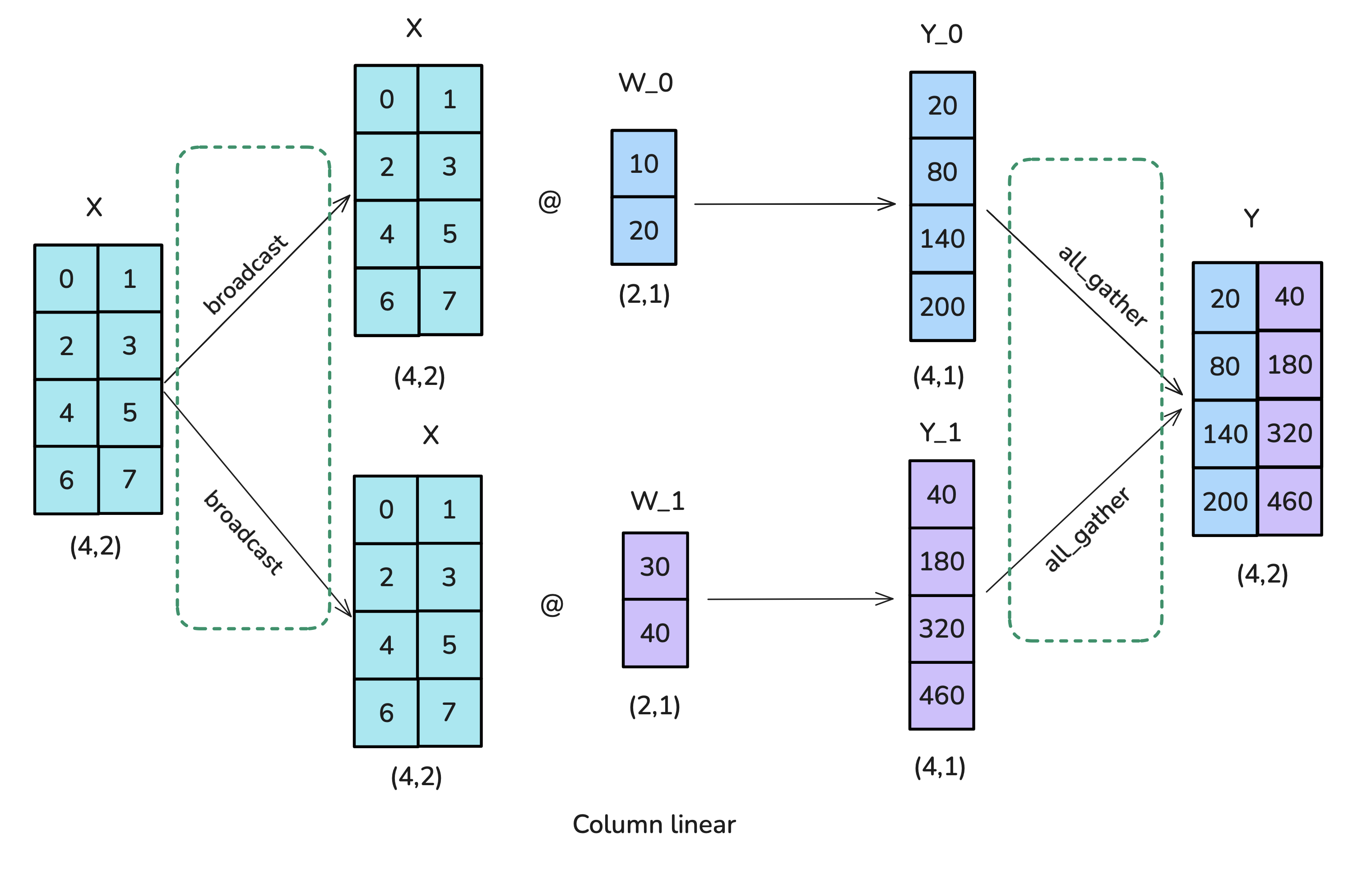
• Column Parallelism: Split weight $A$ column-wise $ [A_1 | … | A_{N_{tp}}]$. Each worker computes $Y_k = f(X A_k)$. Output $Y$ is $[Y_1 | … | Y_{N_{tp}}]$ distributed across workers. Needs AllReduce in backward pass for $\nabla_X$.

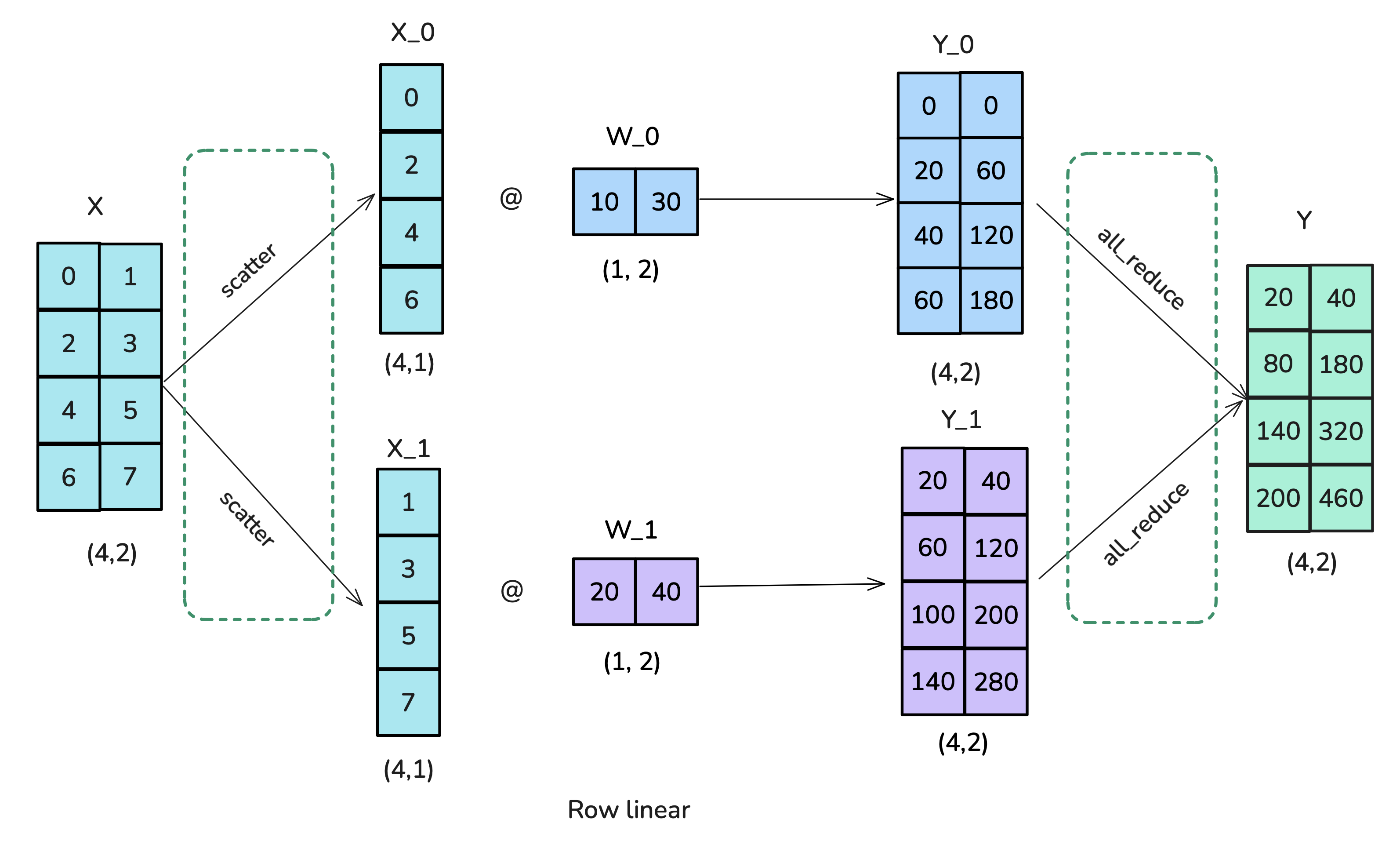
• Row Parallelism: Split weight $A$ row-wise $ [A_1^T | … | A_{N_{tp}}^T]^T$. Input $X$ must also be sharded $[X_1 | … | X_{N_{tp}}]$. Each worker computes $Y_k = f(X_k A_k)$. Final output $Y = \sum Y_k$ requires AllReduce in forward pass.

Reference: Playbook Section

Slide 30: TP Applied to Transformers (FFN & MHA)

Goal: Minimize communication between operations.

FFN ($Y = f(XW_1)W_2$):

1. $W_1$ (expand): Column Parallelism. Input $X$ (replicated), Output $f(Z)$ sharded along intermediate dim $d_{ff}$.
2. $W_2$ (contract): Row Parallelism. Input $f(Z)$ (sharded), Output $Y_k$ partial.
3. Final $Y = \sum Y_k$ via AllReduce.
   • Key: No communication needed between $W_1$ and $W_2$!

MHA:

1. $W_Q, W_K, W_V$: Column Parallelism. Input $X$ (replicated), Outputs $Q_k, K_k, V_k$ sharded (effectively sharding heads).
2. Attention Calc: If $N_{tp}$ divides num heads $a$, each worker computes attention for its local heads using $Q_k, K_k, V_k$. No communication needed here! (Efficient “Head-wise Parallelism”). Output $Attn_k$ sharded.
3. $W_O$: Row Parallelism. Input $Attn_k$ (sharded), Output $Z_k$ partial.
4. Final MHA Output $Y = \sum Z_k$ via AllReduce.

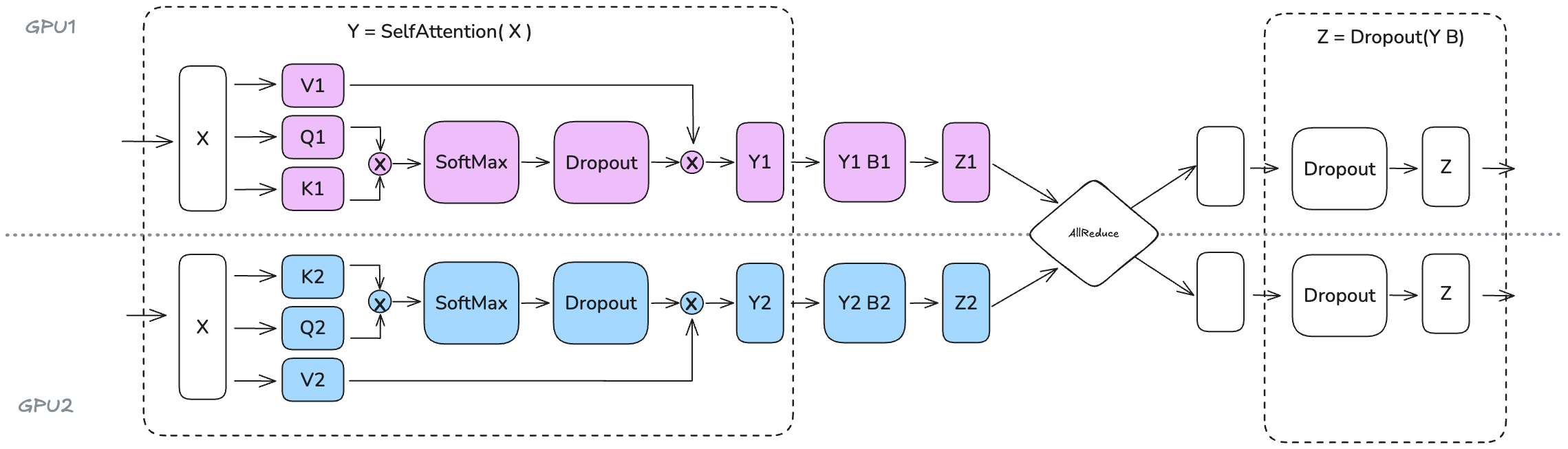(Shows Column for QKV, local attn, Row for Output proj -> AllReduce. Shows Col for FFN1, Row for FFN2 -> AllReduce)

Slide 31: TP Trade-offs

Pros:

• Reduces memory per worker for $w, g, \text{OptState}$ and Activations $A$ (for the parallelized layers).
• Can speed up computation if communication overhead is low.

Cons:

• High Communication Frequency: Requires AllReduce within layer computations. (Shows communication cannot be fully overlapped)
• Needs very high-bandwidth, low-latency interconnect (e.g., NVLink within a node). Usually limited to small $N_{tp}$ (e.g., <= 8).
• Increases implementation complexity.
• Doesn’t parallelize all operations easily (e.g., LayerNorm requires full hidden dim).

Slide 32: Parallelism Strategy 4: Sequence Parallelism (SP)

What: Optimization used with Tensor Parallelism (TP) to reduce activation memory further. Why: TP shards along hidden dim $h$. Operations like LayerNorm, Dropout work on full $h$, preventing activation sharding there. SP shards along sequence dim $s$ for these ops.

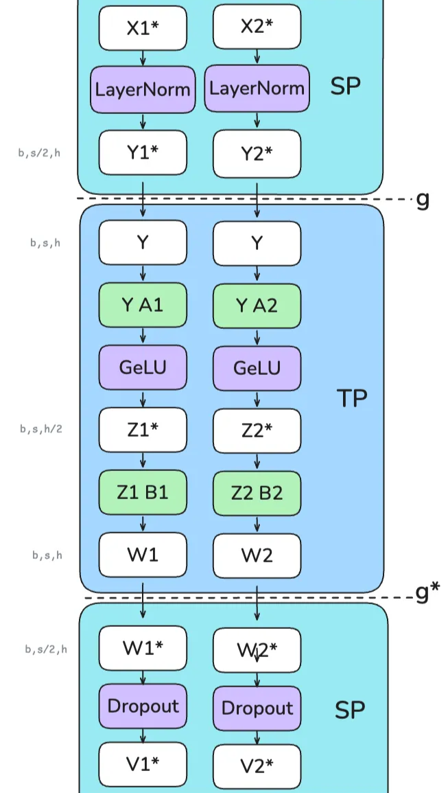
How: Requires communication to switch sharding:

1. SP Region (e.g., LayerNorm): Input $X$ sharded along $s$. Compute LN locally.
2. Transition SP -> TP (g): Use AllGather along $s$ to get full tensor $Y$ (replicated) needed for TP’s column-parallel input.
3. TP Region (e.g., FFN): Compute TP ops (Col-Linear -> Row-Linear). Output is partial $W_k$, sharded along $h$.
4. Transition TP -> SP (g*): Use ReduceScatter along $s$. This sums partial $W_k$ (completing TP’s Row-Linear) AND scatters result along $s$. Output $W^*$ is sharded along $s$.
5. SP Region (e.g., Dropout): Apply Dropout locally to sequence-sharded $W^*$.

Benefit: Reduces peak activation memory by avoiding full $b \times s \times h$ tensor for LN/Dropout. Adds complexity. Communication volume similar to TP, uses AllGather/ReduceScatter instead of AllReduce. Still needs fast interconnect. Reference: Playbook Section

Slide 33: Parallelism Strategy 5: Context Parallelism (CP) & Ring Attention

What: Partition the sequence dimension $s$ globally across $N_{cp}$ workers for most computations. Why: Handle extremely long sequences ($s$) where activations ($b \times s \times h$) become prohibitive, especially in attention ($s^2$).

How:

• Worker $k$ holds sequence chunk $X_k \in \mathbb{R}^{b \times (s/N_{cp}) \times h}$.
• FFN, LN are local.
• Challenge: Attention needs all Keys ($K$) and Values ($V$).
• Solution: Ring Attention:
  1. Workers arranged in a ring.
  2. Repeat $N_{cp}-1$ times:
     • Send current K/V chunk to next worker (async).
     • Compute partial attention with local Q and current K/V chunk (overlap).
     • Receive K/V chunk from previous worker (blocking). Update current K/V.

Communication: Point-to-point K/V passing + final gradient AllReduce across $N_{cp}$. Reference: Playbook Section

Slide 34: CP Challenge: Load Balancing with Causal Masks

Problem: With causal masks (attend only to past) + naive sequential partitioning, workers with early chunks do much less work than workers with late chunks. Bad load imbalance!

(Shows GPU1 has few calcs, GPU4 has many)

Solution: ZigZag Partitioning:

• Assign sequence chunks non-contiguously, mixing early/late tokens on each worker.
• Balances the computation load across all $N_{cp}$ workers.

(Shows computation more evenly distributed)

Benefit: Enables training on very long sequences. Adds complexity to attention.

Slide 35: Parallelism Strategy 6: Pipeline Parallelism (PP)

What: Partition the model layers sequentially into $P$ stages. Stage $p$ runs on worker(s) $p$. Data flows $1 \rightarrow 2 \rightarrow … \rightarrow P$. Why:

• Model parameters $|w|$ too large for single device / TP group.
• Scale across many nodes (TP needs fast intra-node links, PP tolerates slower inter-node links).

How: Stage $p$ computes $A_p = f_p(A_{p-1}; w_p)$. Output $A_p$ is sent to stage $p+1$.

Problem: Pipeline Bubble: Naive sequential execution leaves most stages idle. (Shows large grey idle areas)

Reference: Playbook Section

Slide 36: PP Scheduling: Reducing the Bubble

Idea: Split batch $\mathcal{B}$ into $m$ micro-batches ($\mathcal{B}^{(j)}$). Process them concurrently in the pipeline.

Schedule 1: All-Forward-All-Backward (AFAB / GPipe):

• All micro-batches do full forward pass ($F_1..F_P$).
• Then all micro-batches do full backward pass ($B_P..B_1$).
• Simple, but needs to store activations for all $m$ micro-batches. High activation memory ($\propto m$). Bubble size $\approx (P-1)/m$.

Schedule 2: One-Forward-One-Backward (1F1B / Interleaved):

• Interleave Fwd/Bwd passes more tightly. Start backward pass for micro-batch $j$ as soon as its forward pass finishes.
• Reduces peak activation memory ($\propto P$). Bubble size $\approx (P-1)/m$. More complex.

(Advanced): Interleaved Stages, ZeroBubble schedules exist - more complex, aim for zero bubble.

Slide 37: PP Trade-offs

Pros:

• Partitions very deep models across many devices/nodes.
• Communication (activations/gradients between stages) is less bandwidth-intensive than TP/FSDP collectives, suitable for inter-node networks.

Cons:

• Pipeline Bubble: Inherent inefficiency, limits perfect scaling. Requires large $m$ (many micro-batches, often via gradient accumulation) to amortize.
• Requires careful load balancing (each stage should take similar time).
• Choice of schedule impacts memory and complexity.

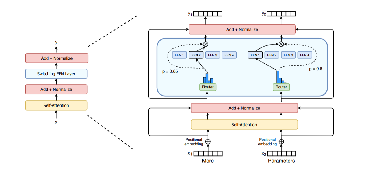
Slide 38: Parallelism Strategy 7: Expert Parallelism (EP)

What: Specialized strategy for Mixture-of-Experts (MoE) models ONLY. Why: Scale models to huge parameter counts by having many specialized “expert” networks (e.g., FFNs), but only activating a few per token.

MoE Layer:

• Replace FFN with $E$ expert FFNs ${f_{e}}$.
• Gating network $R(x_t)$ picks 1 or 2 experts for each token $x_t$.

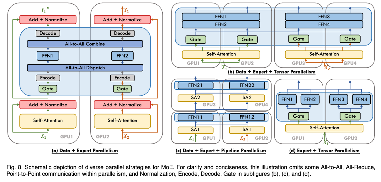
How EP Works:

1. Distribute $E$ experts across $N_{ep}$ workers. Worker $k$ holds experts $E_k$.
2. Gating selects expert $e(x_t)$ for token $x_t$.
3. AlltoAll: Route token $x_t$ to the worker holding expert $e(x_t)$.
4. Worker computes expert output $y_t = f_{e(x_t)}(x_t)$.
5. AlltoAll: Route output $y_t$ back to original worker.

Reference: Playbook Section

Slide 39: EP Trade-offs & Combination with DP

Pros:

• Massive parameter scaling with relatively low compute cost per token (sparse activation).

Cons:

• Only for MoE models.
• High Communication Cost: AlltoAll is communication-intensive, can be a bottleneck. Requires high bisection bandwidth.
• Load balancing challenges (if some experts are chosen more often).

Combination with DP:

• EP alone only parallelizes MoE layers. Non-expert layers are replicated.
• Almost always used with DP ($N_d$ workers) in a 2D grid ($N_d \times N_{ep}$).
  • EP happens across workers in a DP group (row).
  • DP happens across workers holding the same expert shards (column).

Slide 40: Combining Strategies: The Need for Hybrid Parallelism

No Silver Bullet! Each strategy has strengths and weaknesses.

• DP/ZeRO: Scales data throughput, limited by activation memory (DP) or communication (ZeRO).
• TP/SP/CP: Reduces activation/param memory per device, needs fast interconnect, limited scalability.
• PP: Scales deep models across nodes, suffers from bubble.
• EP: Scales MoE parameters, needs AlltoAll.

Solution: Combine them! Leverage hardware topology.

Common Combo: 3D Parallelism ($N = N_d \times P \times N_{tp}$)

• TP ($N_{tp}$): Within a node (uses NVLink). Partitions layers/activations.
• PP ($P$): Across nodes (uses inter-node network). Partitions layers sequentially.
• DP ($N_d$): Across nodes/racks. Replicates the PP+TP setup, processes different data.

Reference: Playbook Section

Slide 41: Role of FSDP (ZeRO-3) in Combined Strategies

• In 3D (or higher) parallelism, the “DP” dimension ($N_d$) is often implemented using FSDP (ZeRO-3) instead of standard DP.
• Why? FSDP shards parameters/gradients/optimizer states across the $N_d$ replicas.
• Benefit: Drastically reduces memory per worker compared to replicating the model state in standard DP. Allows fitting much larger models within the combined (FSDP + PP + TP) setup.

PP vs. FSDP Parameter Partitioning:

• PP: Partitions layer-wise into sequential stages. Worker $p$ holds full parameters $w_p$ for its layers. Communicates activations. Sensitive to bubble (needs high grad_acc $m$).
• FSDP: Partitions parameter-wise across DP workers. Worker $k$ holds shards $w^{(k)}$ from all layers. Communicates parameter shards (AllGather). Sensitive to overlap (needs large micro-batch mbs or sequence length s).

(Combining PP and FSDP is possible but complex, needs large global batch size).

Slide 42: Adding CP & EP to the Mix (Conceptual 5D)

• CP (Context Parallelism): Added when sequences ($s$) are very long. Typically partitions along DP or PP dimension workers, adds Ring Attention communication.
• EP (Expert Parallelism): Added only for MoE models. Distributes experts, often along DP dimension workers, adds AlltoAll communication.

(Conceptual diagram showing how DP, PP, TP, EP, CP dimensions relate)

Slide 43: Summary Table of Parallelism Strategies

(The table summarizing What, Granularity, Communication, Pros, Cons for DP, ZeRO, PP, TP, EP)

Key Takeaway: Choosing the right mix depends on model size, architecture (MoE?), sequence length, hardware (GPU memory, interconnects), and desired batch size.

Slide 44: Finding the Best Configuration (Iterative Process)

General Approach: (From Playbook)

1. Fit in Memory:
   • Start with minimal setup (1 node).
   • Add necessary partitioning: TP (intra-node), PP (inter-node), FSDP (across DP dim) until model parameters fit. Use ZeRO stage appropriate for memory needs.
   • Use Activation Recomputation aggressively if activations are the bottleneck.
2. Scale Batch Size:
   • Increase DP/FSDP degree ($N_d$).
   • Use Gradient Accumulation ($A$) to reach target global batch size ($GBS = N_d \times \text{per_replica_batch} \times A$).
   • Add CP if sequence length ($s$) is limiting factor.
3. Optimize Throughput (MFU/TFLOPS):
   • Tune micro-batch sizes (for PP schedule, FSDP overlap).
   • Maximize TP degree within node constraints.
   • Balance PP stages for minimal bubble.
   • Profile and identify communication vs. computation bottlenecks.

Reference: Playbook Section

Slide 45: Conclusion

• Training large Transformers requires overcoming single-device memory/compute limits.
• Activation Memory is often the primary bottleneck, addressed by Activation Recomputation.
• Parallelism Strategies distribute the workload:
  • DP/FSDP: Distributes data/model state.
  • TP/SP/CP: Distributes layer computation / activations.
  • PP: Distributes layers sequentially.
  • EP: Distributes MoE experts.
• State-of-the-art training uses combinations (e.g., FSDP + PP + TP) tailored to the model and hardware.
• Understanding communication primitives (AllReduce, AllGather, etc.) and trade-offs (memory vs. compute vs. communication) is crucial.
• Resources like the Ultrascale Playbook are invaluable guides.