Stochastic Optimization Basics in 1D

Slide 1: Training as Optimization

Purpose: Frame the lecture as training by minimizing a loss.

We have labeled data and want a rule that predicts future labels.
We treat the model class as fixed and focus on training it.
We work in 1D to keep the mechanism visible.

Slide 2: Labeled Data

Purpose: Fix the training data notation.

Formula:

\[(x_1,y_1),\ldots,(x_n,y_n)\]

Example: $x_i$ is an email and $y_i \in {0,1}$ is a spam label.

Slide 3: What Is a Model?

Purpose: Define the object we are training.

Formula:

\[m(x;w)\]

$w$ is the parameter (weights); here $w \in \mathbb{R}$.
The same pipeline applies in higher dimensions.

Slide 4: Model Class Choices

Purpose: Separate a single model from a class of models.

We pick a class $\mathcal{M}$ and then search inside it.
Extreme 1: a constant model that predicts the majority label.
Extreme 2: a large parametric family (e.g., neural nets) with architecture choices.

Slide 5: Three Questions

Purpose: Separate optimization, model selection, and generalization.

Optimization: for a fixed model, how do we choose $w$?
Learning: among $\mathcal{M}$, which trained model do we pick?
Generalization: how well will the chosen model do on new data?

Slide 6: Train-Validation-Test Split

Purpose: State the standard workflow.

Training set: fit parameters $w$ for each candidate model.
Validation set: choose hyperparameters (step size, batch size, architecture).
Test set: estimate out-of-sample performance of the final choice.

Slide 7: Test-Set Leakage

Purpose: Warn against treating the test set as untouchable.

Repeatedly adapting to test performance turns it into validation.
Kaggle-style third-party scoring still leaks signal if you iterate.
In practice I often merge validation and test into a small holdout to maximize training data.

Slide 8: Training Loss (Empirical Risk)

Purpose: Define the objective we minimize.

Formula:

\[L(w) = \frac{1}{n}\sum_{i=1}^n \ell_i(w)\]

$\ell_i(w)$ is the per-sample loss.

Slide 9: Training Objective

Purpose: State the optimization problem.

Formula:

\[\min_{w \in \mathbb{R}} L(w)\]

Same objective as in Lecture 1; the new issue is scale.

Slide 10: Full Gradient

Purpose: Show the cost of a full-batch step.

Formula:

\[L'(w) = \frac{1}{n}\sum_{i=1}^n \ell_i'(w)\]

Computing $L’(w)$ touches all $n$ samples.

Slide 11: Why Stochastic Methods

Purpose: Motivate SGD by scale.

The cost of a full gradient scales linearly with $n$.
For modern language models, $n$ can be on the order of trillions.
Even a single full gradient can be too expensive.

Slide 12: SGD Update

Purpose: State the stochastic update rule.

Formula:

\[w_{k+1} = w_k - \eta\,\ell_{i_k}'(w_k)\]

$\eta>0$ is the step size.
$i_k$ is sampled uniformly from ${1,\ldots,n}$.

Slide 13: Sampling a Random Index (PyTorch)

Purpose: Show how to draw one sample index in code.

Random index in ${0,1,\ldots,n-1}$.

i_k = torch.randint(low=0, high=n, size=(1,)).item()

Slide 14: Sampling a Minibatch (PyTorch)

Purpose: Show how to sample a batch with replacement.

idx = torch.randint(low=0, high=n, size=(B,))

Slide 15: Per-Step Cost

Purpose: Compare full-batch GD to SGD.

Full-batch GD: one step costs $n$ sample gradients.
SGD (batch size 1): one step costs 1 sample gradient.
The key question is whether this cheaper update still makes progress.

Slide 16: Synthetic Data for the Experiment

Purpose: Define the regression dataset.

$x_i \sim \mathrm{Unif}[-1,1]$.
$y_i = x_i + \sigma g_i$.
$g_i \sim \mathcal{N}(0,1)$ independent.
$\sigma$ controls label noise.

Slide 17: Linear Model

Purpose: Fix the prediction rule.

Formula:

\[\hat y = m(x;w) = wx\]

Slide 18: Per-Sample Loss

Purpose: Define the squared error.

Formula:

\[\ell_i(w) = \tfrac{1}{2}(y_i - wx_i)^2\]

Slide 19: Per-Sample Derivative

Purpose: Compute the stochastic gradient.

Formula:

\[\ell_i'(w) = (wx_i - y_i)x_i\]

Slide 20: SGD Update for This Problem

Purpose: Write the concrete 1D update.

Formula:

\[w_{k+1} = w_k - \eta (w_k x_{i_k} - y_{i_k}) x_{i_k}\]

Slide 21: Closed-Form Minimizer (Diagnostics Only)

Purpose: Provide the reference solution for the toy problem.

Formula:

\[w^\star = \frac{\sum_{i=1}^n x_i y_i}{\sum_{i=1}^n x_i^2}\]

In real ML this closed form usually does not exist.

Slide 22: Objective Gap

Purpose: Define the diagnostic we will plot.

Use $L(w_k)-L(w^\star)$ as the objective gap.
This is only feasible because $w^\star$ is known here.

Slide 23: What Success Looks Like

Purpose: See the fitted line on noisy data.

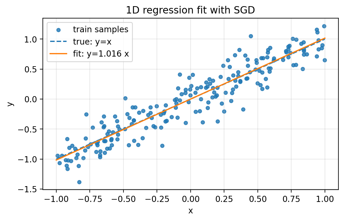SGD fit on synthetic regression data Figure 2.1.

Slide 24: Constant Step Size Behavior

Purpose: Describe the noise-floor phenomenon.

On noisy data, the objective drops quickly then stabilizes.
Larger $\eta$ often reduces the loss faster at first.
Smaller $\eta$ reaches a lower noise floor.

Slide 25: Constant Step Size Tradeoff

Purpose: Visualize the noise floor across step sizes.

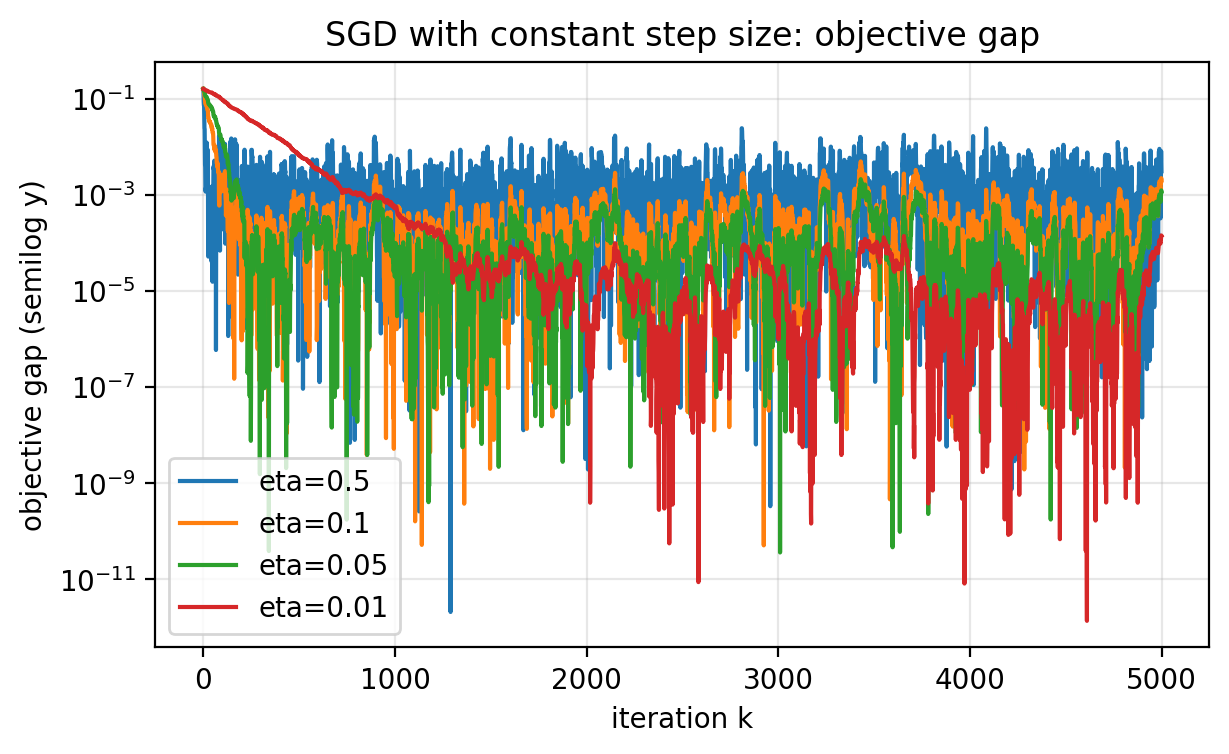SGD constant step size: objective gap Figure 2.2.

Slide 26: What “Noise Floor” Means

Purpose: Clarify the diagnostic.

The floor is the rough level where the curve bottoms out on average.
You still see sharp downward jumps.
There is no sustained downward trend beyond that level.

Slide 27: Full-Dataset Diagnostics

Purpose: Explain what we can log in the toy problem.

Full training loss $L(w_k)$.
Full gradient magnitude $|L’(w_k)|$.
Use torch.no_grad() when computing these.
At scale this is too expensive to do every step.
You cannot detect and keep only the rare low-loss iterates.

Slide 28: Diagnostics Plot

Purpose: Show objective gap and gradient norm together.

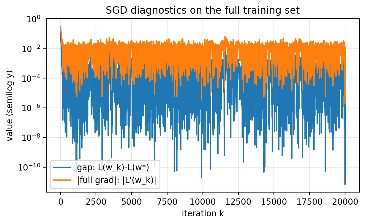SGD diagnostics: objective gap and full gradient magnitude Figure 2.3.

Slide 29: Convergent Step Size Schedules

Purpose: State the classical sufficient condition.

Formula:

\[\sum_{k=0}^\infty \eta_k = \infty \quad\text{and}\quad \sum_{k=0}^\infty \eta_k^2 < \infty\]

Slide 30: Power Schedule

Purpose: Give a standard schedule that satisfies the condition.

Formula:

\[\eta_k = \frac{\eta_0}{(k+1)^p} \quad\text{with}\quad p \in (\tfrac{1}{2},1]\]

Slide 31: Geometric Schedule

Purpose: Give a fast-decaying alternative.

Formula:

\[\eta_k = \eta_0 \gamma^k \quad\text{with}\quad \gamma \in (0,1)\]

Often decays too quickly and progress freezes.

Slide 32: Schedule Comparison

Purpose: Compare constant, geometric, and power schedules.

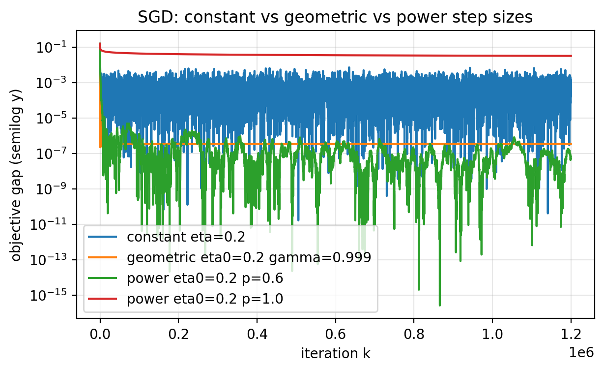Step size schedules Figure 2.4.

Slide 33: Unbiased Gradient Estimate

Purpose: Explain why SGD points in the right direction on average.

Formula:

\[\mathbb{E}[X] = \frac{1}{n}\sum_{i=1}^n \ell_i'(w) = L'(w)\]

Here $X=\ell_i’(w)$ with $i$ uniform on ${1,\ldots,n}$.

Slide 34: Expected Update

Purpose: Link SGD to gradient descent in expectation.

Formula:

\[\mathbb{E}[w_{k+1}\mid w_k] = w_k - \eta L'(w_k)\]

Slide 35: Variance Controls the Noise Floor

Purpose: Explain what higher label noise does.

Larger $\sigma$ increases the variance of sample gradients.
Same step size leads to more jitter and a higher noise floor.
Progress toward low error slows down.

Slide 36: Effect of Label Noise

Purpose: Visualize variance effects.

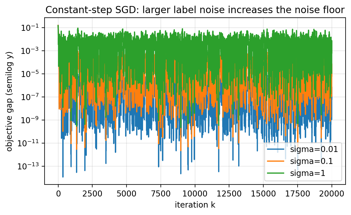Effect of label noise on SGD Figure 2.6.

Slide 37: Variance Reduction by Averaging

Purpose: State the basic probability fact.

Formula:

\[\mathrm{Var}\Big(\frac{1}{B}\sum_{j=1}^B X_j\Big) = \frac{1}{B}\,\mathrm{Var}(X_1)\]

Slide 38: Minibatch Gradient Estimate

Purpose: Define the minibatch estimator.

Formula:

\[G_k = \frac{1}{B}\sum_{i \in B_k} \ell_i'(w_k)\]

Sample a minibatch $B_k \subset {1,\ldots,n}$ of size $B$.
Update: $w_{k+1} = w_k - \eta G_k$.

Slide 39: Rule of Thumb for Noise

Purpose: Connect batch size and step size.

The noise level scales like $\eta/B$.
To match batch-1 noise, keep $\eta/B$ approximately constant.

Slide 40: Two Ways to Measure Progress

Purpose: Separate iteration count from total gradient work.

Iterations: $k$.
Total gradients: $kB$.
These two views can tell different stories.

Slide 41: Minibatch vs Iterations

Purpose: Show iteration efficiency.

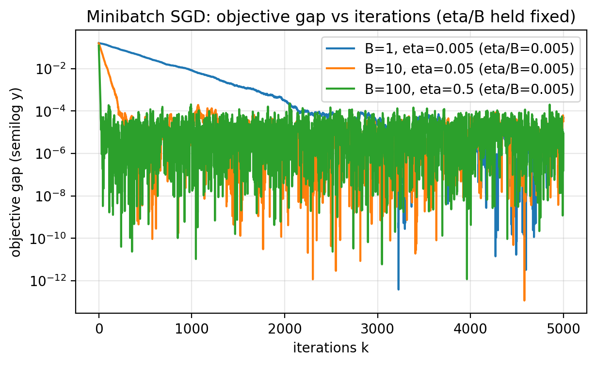Minibatch: objective gap vs iterations Figure 2.7.

Slide 42: Minibatch vs Total Gradients

Purpose: Compare total gradient work.

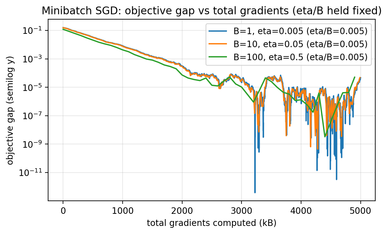Minibatch: objective gap vs total gradients Figure 2.8.

Slide 43: Why Use Large Batches

Purpose: Motivate minibatches via parallelism.

If $B$ gradients are computed in parallel, wall-clock time per step can stay near batch-1.
Then fewer iterations can mean faster time-to-result.

Slide 44: When Constant Steps Are Enough

Purpose: State a clean sufficient condition.

Formula:

\[\ell_i'(w^\star)=0 \quad \text{for all } i\]

Each per-sample gradient vanishes at the optimum.

Slide 45: Noiseless Regression Example

Purpose: Show a case where the condition holds.

Formula:

\[y_i = x_i\]

Then $w^\star = 1$.

Slide 46: Per-Sample Gradients Vanish

Purpose: See why SGD becomes deterministic.

Formula:

\[\ell_i'(w) = (w-1)x_i^2\]

At $w=1$, each $\ell_i’(1)=0$.
Even a constant step size like $\eta=0.5$ converges quickly here.

Slide 47: Noiseless vs Noisy

Purpose: Contrast the two regimes.

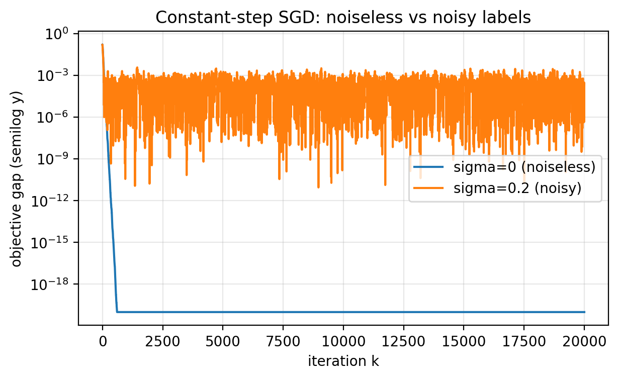Noiseless vs noisy: constant step size Figure 2.5.

Slide 48: Expressivity Context

Purpose: Explain when constant steps are common in practice.

Classical ML models often cannot fit noisy data exactly.
Deep nets can often interpolate noisy labels.
Constant step sizes can be acceptable in highly expressive models.

Slide 49: Validation Loss

Purpose: Monitor performance on new data.

Training loss is not the goal; we care about new inputs.
Define $L_{\mathrm{val}}(w)$ by averaging the same loss on a validation set.
Evaluate periodically, not every iteration.
Use torch.no_grad() during evaluation.

Slide 50: Validation Loop (PyTorch)

Purpose: Show the evaluation pattern.

# Assume we have training data (x_tr, y_tr) and validation data (x_va, y_va).
# Assume "step(w)" performs one SGD or minibatch-SGD update on training data.

eval_every = 200

for k in range(max_iters):
    w = step(w)

    if k % eval_every == 0:
        with torch.no_grad():
            train_loss = 0.5 * torch.mean((y_tr - w * x_tr)**2)
            val_loss = 0.5 * torch.mean((y_va - w * x_va)**2)

        print(f"k={k:6d}  train_loss={train_loss:.3e}  val_loss={val_loss:.3e}")

Slide 51: Why Monitor Validation Loss

Purpose: State what validation diagnostics are for.

Detect divergence early (step size too large).
Choose among hyperparameters (step size, schedule, batch size).
Stop when validation loss plateaus.
Validation loss is optimistic because you tune against it.

Slide 52: Conclusion: Core Points

Purpose: Capture the main takeaways.

Training a model is empirical risk minimization.
Full gradients cost $n$ sample gradients; SGD uses 1 per step.
Constant-step SGD on noisy data stabilizes at a noise floor.
Step size schedules that decrease can drive error lower but can be slow.
Unbiasedness points in the right direction; variance makes progress noisy.

Slide 53: Conclusion: Practical Points

Purpose: Capture the practical takeaways.

Minibatches reduce variance by averaging gradients and improve iteration efficiency.
Fair comparisons must account for total gradient computations and parallelism.
Diagnostics should include validation loss, not just training loss.
These insights carry over to higher-dimensional models.