2. Stochastic Optimization Basics in 1D

Motivation: training a model means minimizing a loss
Empirical risk: the training objective
SGD: replace a full gradient with a sample gradient
Experiment: 1D linear regression with noisy labels
Step sizes: constant steps hit a noise floor
Step size schedules that converge
Why SGD works at all: unbiasedness and variance
Minibatches: variance reduction and parallelism
When constant steps are enough
Diagnostics: monitor validation loss, not just training loss
Conclusion
Appendix: code to generate all figures

1. Motivation: training a model means minimizing a loss

We have labeled data:

\[(x_1,y_1),\ldots,(x_n,y_n).\]

Example: $x_i$ is an email and $y_i \in {0,1}$ is a spam label.

We expect to see more inputs $x$ in the future without labels. The point of training is to pick a rule that predicts $y$ from $x$ as well as possible.

What is a “model”?

A model is a parametric mapping from inputs to predictions:

\[m(x;w).\]

$w$ is the parameter vector (often called weights).
In this lecture we work with a single parameter $w \in \mathbb{R}$.
The same pipeline applies in higher dimensions.

Which models are we allowed to choose?

In practice we pick a class of models $\mathcal{M}$, then we search inside that class.

Two extremes:

A “constant model” that always predicts the majority label.
A large parametric family, like neural networks, where you also need to decide architecture (layers, width, etc.).

In this lecture we treat the model class $\mathcal{M}$ as fixed. We focus on the optimization subproblem: how to train a chosen model by minimizing a loss.

Training vs choosing a model vs testing

There are three distinct questions.

Optimization (training): for a fixed model, how do we choose $w$?
Learning (model selection): among a class $\mathcal{M}$, which trained model do we pick?
Generalization: how well will the chosen model do on new data?

The standard workflow is a train-validation-test split.

Training set: used to fit parameters $w$ for each candidate model.
Validation set: used to choose among models and hyperparameters (step size, batch size, architecture).
Test set: held out to estimate out-of-sample performance of the final choice.

One might think the “test set” is a sacred object. However, if you repeatedly look at test performance and adapt, you have effectively turned the test set into a validation set.

Sometimes test data is held by a neutral third party (e.g., Kaggle) that only reports a score. Even then you can still adapt to that feedback; see my note on the ladder mechanism for ML competitions.

In practice I often merge validation and test into a single holdout set and keep it small so more data goes into training, then use that holdout to choose hyperparameters like network depth.

2. Empirical risk: the training objective

Fix a training set $(x_i,y_i)$.

A standard setup is:

Define a per-sample loss $\ell_i(w)$.
Average over the training set to get the training loss (empirical risk)

\[L(w) = \frac{1}{n}\sum_{i=1}^n \ell_i(w).\]

Training is the optimization problem

\[\min_{w \in \mathbb{R}} L(w).\]

This is the same empirical-risk objective as in the previous lecture; the new issue is scale.

If we run full-batch gradient descent, we need the derivative of the average loss,

\[L'(w) = \frac{1}{n}\sum_{i=1}^n \ell_i'(w).\]

The cost of computing $L’(w)$ scales linearly with $n$, because you must touch all $n$ samples.

For modern language models, $n$ can be on the order of trillions. Even a single full gradient can be too expensive. This is where stochastic gradient methods enter.

3. SGD: replace a full gradient with a sample gradient

Stochastic gradient descent (SGD) is a modification of gradient descent.

Choose a step size (learning rate) $\eta>0$.
At iteration $k$, sample an index $i_k \in {1,\ldots,n}$ uniformly at random.
Update using a single sample derivative:

\[w_{k+1} = w_k - \eta\,\ell_{i_k}'(w_k).\]

Sampling a random index in PyTorch

If your dataset has length n and you want a random index in {0,1,...,n-1}:

i_k = torch.randint(low=0, high=n, size=(1,)).item()

A minibatch of size B (sampling with replacement) is:

idx = torch.randint(low=0, high=n, size=(B,))

The computational point is immediate.

Full-batch GD: one step costs $n$ sample-gradients.
SGD (batch size 1): one step costs 1 sample-gradient.

The question is whether this cheaper update still makes progress.

4. Experiment: 1D linear regression with noisy labels

We will fit a scalar linear model on synthetic data.

Data

Generate $n$ training points:

$x_i \sim \mathrm{Unif}[-1,1]$,
$y_i = x_i + \sigma g_i$,
$g_i \sim \mathcal{N}(0,1)$ independent.

Here $\sigma$ controls label noise.

Model and loss

Model:

\[\hat y = m(x;w) = wx.\]

Per-sample squared loss:

\[\ell_i(w) = \tfrac{1}{2}(y_i - wx_i)^2.\]

Derivative:

\[\ell_i'(w) = (wx_i - y_i)x_i.\]

So SGD becomes

\[w_{k+1} = w_k - \eta (w_k x_{i_k} - y_{i_k}) x_{i_k}.\]

A closed-form minimizer exists (but we will use it only for diagnostics)

The training loss is a quadratic in $w$, so the minimizer is

\[w^\star = \frac{\sum_{i=1}^n x_i y_i}{\sum_{i=1}^n x_i^2}.\]

In real ML, we usually do not have a closed form minimizer. Here we do, so we will use it to compute an “objective gap” diagnostic $L(w_k)-L(w^\star)$.

What “success” looks like in this toy problem

The fitted model is a line. After training, we want the line $y=wx$ to match the trend in the data.

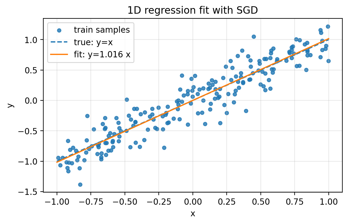SGD fit on synthetic regression data Figure 2.1: Synthetic 1D regression data (scatter), the true relationship $y=x$ (dashed), and the fitted line $y=\hat w x$ produced by SGD (solid).

5. Step sizes: constant steps hit a noise floor

Fix a constant step size $\eta$.

On noisy data ($\sigma>0$), the objective typically decreases quickly at first, then it stops improving past a threshold. This is the noise floor behavior.

Two consistent empirical facts:

Larger $\eta$ often reduces the loss faster at the beginning.
Smaller $\eta$ reaches a lower noise floor.

The trade-off is visible below.

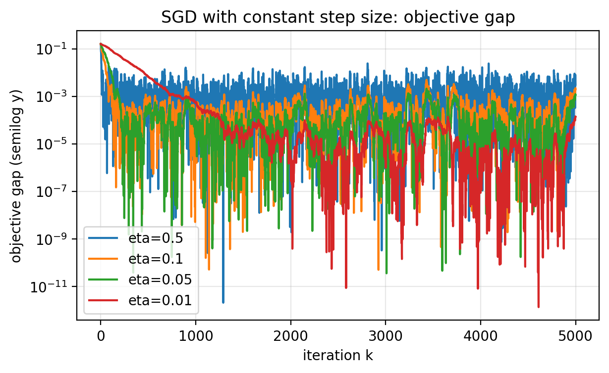SGD constant step size: objective gap Figure 2.2: Objective gap $L(w_k)-L(w^\star)$ for several constant step sizes on the same dataset. Larger step sizes move quickly at first but stabilize at higher error. Smaller step sizes move more slowly but reach a lower noise floor. The curves fluctuate because the iterates $w_k$ fluctuate.

The term “noise floor” refers to the rough level where the curve bottoms out on average. You still see occasional sharp downward jumps, but there is no sustained downward trend past that level.

Diagnostics (and why they are “cheating” at scale)

In this toy problem, it is easy to log:

the full training loss $L(w_k)$,
the full training gradient magnitude $|L’(w_k)|$.

This is useful for debugging, but it defeats the point of SGD when $n$ is large, because evaluating $L(w)$ and $L’(w)$ requires looping over the entire dataset.

When you do compute these diagnostics, do it under torch.no_grad() so PyTorch does not build graphs you will never backprop through.

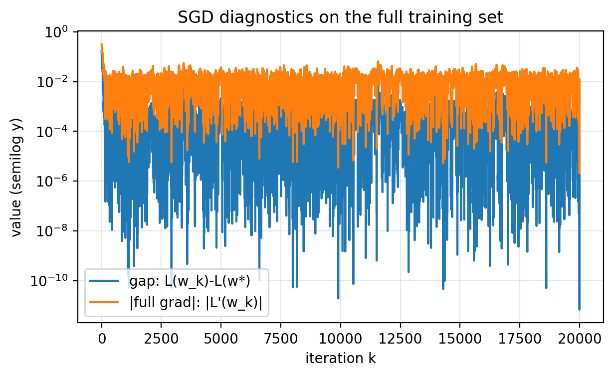SGD diagnostics: objective gap and full gradient magnitude Figure 2.3: Two full-dataset diagnostics: $L(w_k)-L(w^\star)$ and $|L’(w_k)|$. Both flatten to a noise floor. These are informative in a toy problem. For large $n$, computing them every step is too expensive.

In large-scale training, you typically cannot compute the full objective gap or gradient every iteration, so you cannot detect and keep only the rare low-loss iterates when a downward spike happens.

6. Step size schedules that converge

A constant step size keeps injecting noise forever. If you want convergence to high precision, you usually need $\eta_k \to 0$.

A classical sufficient condition for stochastic approximation is:

\[\sum_{k=0}^\infty \eta_k = \infty \quad\text{and}\quad \sum_{k=0}^\infty \eta_k^2 < \infty.\]

A common choice that satisfies this is a power law:

\[\eta_k = \frac{\eta_0}{(k+1)^p} \quad\text{with}\quad p \in (\tfrac{1}{2},1].\]

A geometric schedule

\[\eta_k = \eta_0 \gamma^k \quad\text{with}\quad \gamma \in (0,1)\]

also goes to zero, but often too quickly: after some point the steps become negligible and progress effectively stops.

The next figure compares a constant step size, a geometric schedule, and power schedules over a long horizon.

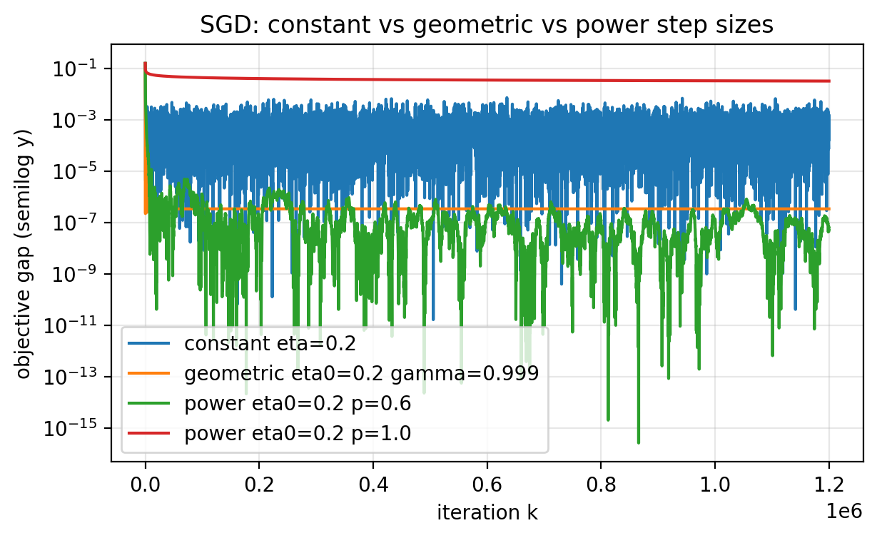Step size schedules Figure 2.4: Constant step size hits a noise floor. A geometric schedule can decay so quickly that it “freezes” early. Power schedules $\eta_k=\eta_0/(k+1)^p$ with $p \in (\tfrac{1}{2},1]$ keep making progress and can drive the objective gap down further, at the cost of slower long-run movement.

7. Why SGD works at all: unbiasedness and variance

SGD works because the stochastic gradient is an unbiased estimate of the full gradient.

Let $i$ be uniform on ${1,\ldots,n}$. Define the random variable

\[X = \ell_i'(w).\]

Then

\[\mathbb{E}[X] = \frac{1}{n}\sum_{i=1}^n \ell_i'(w) = L'(w).\]

So the expected update matches a gradient descent update:

\[\mathbb{E}[w_{k+1}\mid w_k] = w_k - \eta L'(w_k).\]

Unbiasedness is not the full story. The variance of the gradient estimator controls how noisy the iterates are and how quickly you can settle down.

In the regression model above, increasing $\sigma$ increases the noise in the labels, which increases the variance of sample gradients. With the same step size, larger $\sigma$ produces:

more jitter in the iterates,
a higher noise floor,
slower progress toward low error.

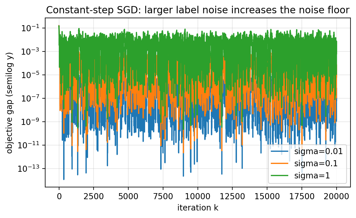Effect of label noise on SGD Figure 2.6: Larger label noise $\sigma$ increases the variance of sample gradients, which raises the noise floor and makes the trajectory noisier for the same step size.

8. Minibatches: variance reduction and parallelism

Variance reduction is the simplest lever you can pull.

A basic probability fact:

If $X_1,\ldots,X_B$ are iid with variance $\mathrm{Var}(X_1)$, then

\[\mathrm{Var}\Big(\frac{1}{B}\sum_{j=1}^B X_j\Big) = \frac{1}{B}\,\mathrm{Var}(X_1).\]

A minibatch gradient is exactly this kind of average.

Minibatch SGD

At iteration $k$:

Sample a minibatch $B_k \subset {1,\ldots,n}$ of size $B$.
Form the minibatch gradient estimate

\[G_k = \frac{1}{B}\sum_{i \in B_k} \ell_i'(w_k).\]

Update

\[w_{k+1} = w_k - \eta G_k.\]

The rule of thumb from this lecture is:

the “noise level” scales like $\eta/B$.

So if you want minibatch SGD (batch size $B$) to have a similar noise floor to batch size 1, you scale step sizes so that $\eta/B$ is approximately constant.

Iterations versus total gradient computations

One might think larger minibatches are always better because they converge in fewer iterations. However, each iteration costs $B$ gradients.

A more honest x-axis is total gradients computed so far, which is $kB$ after $k$ iterations.

Below we show the same experiment two ways:

x-axis = iterations $k$,
x-axis = total gradients $kB$.

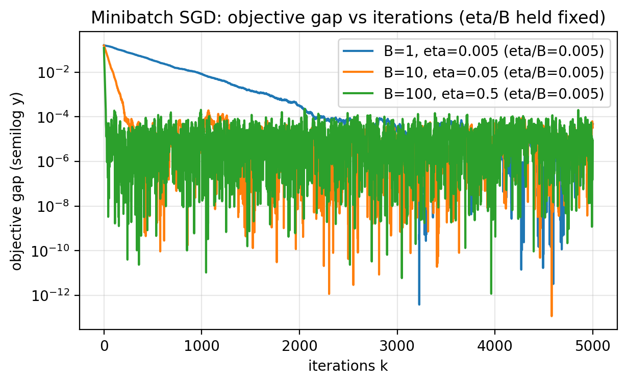Minibatch: objective gap vs iterations Figure 2.7: With step sizes scaled so that $\eta/B$ is constant, larger batches reach the same error in fewer iterations. This is iteration efficiency, not necessarily sample efficiency.

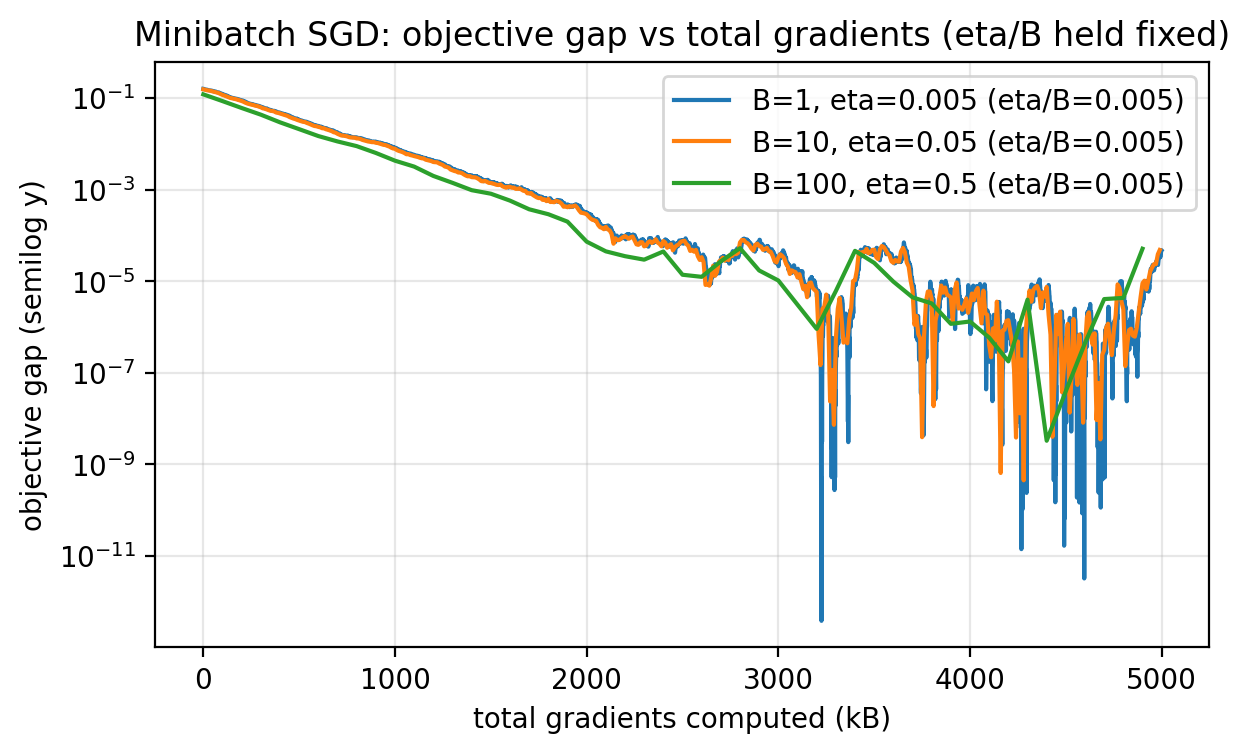Minibatch: objective gap vs total gradients Figure 2.8: Replotting against total gradient computations $kB$ shows that minibatching does not magically reduce total gradient work. It mainly trades fewer iterations for more work per iteration.

Why use large batches at all?

Parallelism.

If you can compute the $B$ sample gradients in parallel (e.g., on a GPU), then a minibatch step can take close to the wall-clock time of a batch-1 step.

In that case, Figure 2.7 is the relevant one: fewer iterations can mean faster time-to-result.

9. When constant steps are enough

Constant step size does not always imply a noise floor.

A clean sufficient condition is: at the optimum, the per-sample gradients vanish, not just the average gradient.

In our regression setup, if the data are noiseless,

\[y_i = x_i,\]

then $w^\star=1$ and for every sample

\[\ell_i'(w) = (wx_i - y_i)x_i = (w-1)x_i^2.\]

At $w=1$, each $\ell_i’(1)=0$. There is no gradient noise at the optimum. SGD behaves like a stable deterministic method and can converge all the way. In this toy problem, even a constant step size like $\eta=0.5$ converges quickly when labels are noiseless.

With label noise ($\sigma>0$), the residuals never vanish, so the sample gradients do not vanish at the optimum. The gradient estimator has nonzero variance even at $w^\star$, and constant-step SGD keeps bouncing.

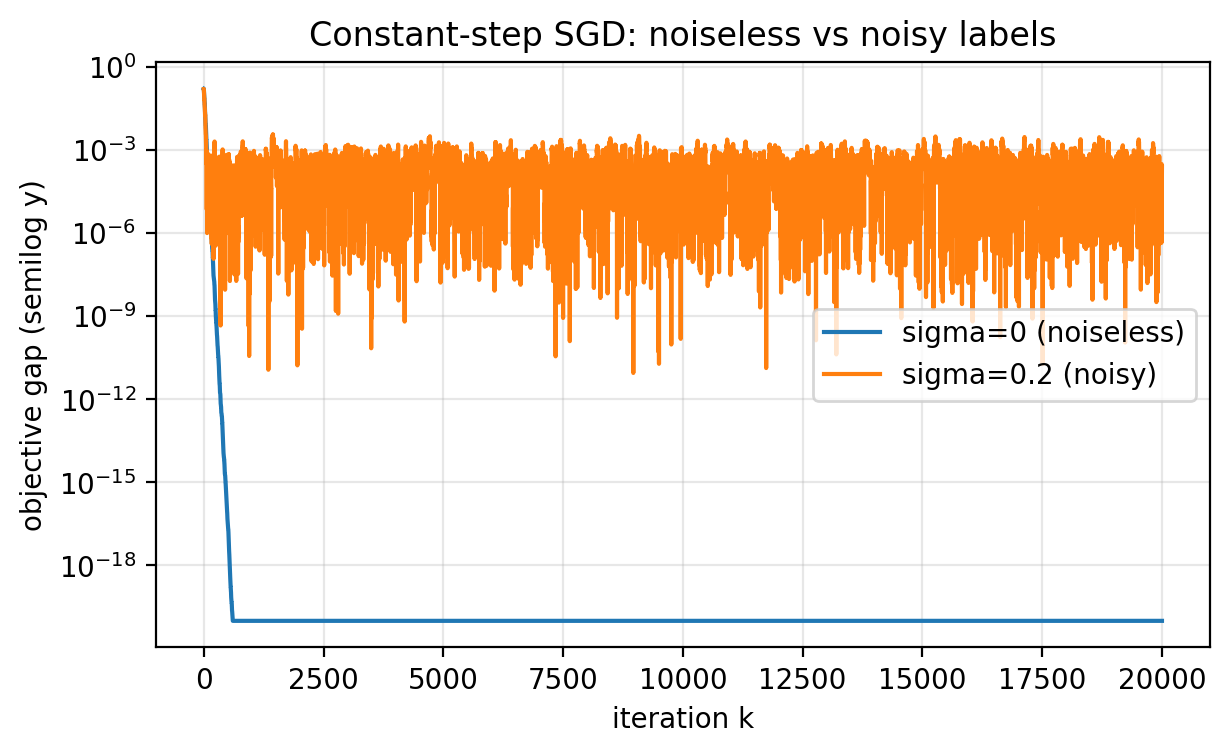Noiseless vs noisy: constant step size Figure 2.5: With noiseless labels, constant-step SGD can converge to high precision because every sample gradient vanishes at the optimum. With noisy labels, constant-step SGD stabilizes at a nonzero noise floor.

Which regime is more common depends on model expressivity. In classical machine learning, models are often too simple to fit noisy data exactly, so constant-step SGD still sees gradient noise. In deep learning, models can often interpolate even noisy labels, so constant step sizes are frequently acceptable in practice. It is still useful to keep both regimes in mind.

10. Diagnostics: monitor validation loss, not just training loss

Training loss is not the end goal. We care about performance on new data.

A standard diagnostic is the validation loss:

form $L_{\mathrm{val}}(w)$ by averaging the same per-sample loss over a validation set,
evaluate it periodically during training.

Two mechanics matter in PyTorch:

Validation evaluation should run under torch.no_grad() so you do not build computation graphs.
You usually do not evaluate every iteration. You pick an eval_every interval.

A schematic loop:

# Assume we have training data (x_tr, y_tr) and validation data (x_va, y_va).
# Assume "step(w)" performs one SGD or minibatch-SGD update on training data.

eval_every = 200

for k in range(max_iters):
    w = step(w)

    if k % eval_every == 0:
        with torch.no_grad():
            train_loss = 0.5 * torch.mean((y_tr - w * x_tr)**2)
            val_loss = 0.5 * torch.mean((y_va - w * x_va)**2)

        print(f"k={k:6d}  train_loss={train_loss:.3e}  val_loss={val_loss:.3e}")

Why monitor validation loss?

detect divergence early (step size too large),
choose among hyperparameters (step size, schedule, batch size),
stop training when the validation loss plateaus.

Validation loss is usually optimistic, because you tune hyperparameters against it, so it tends to understate true out-of-sample error.

11. Conclusion

What you should take from this lecture:

Training a model is usually empirical risk minimization: minimize an average loss.
Full gradients cost $n$ sample-gradients. SGD reduces this to 1 sample-gradient per step.
Constant-step SGD on noisy data typically stabilizes at a noise floor.
Step size schedules $\eta_k \to 0$ can drive the error lower, but they can be slow.
Unbiasedness explains why SGD points in the right direction on average. Variance explains why progress is noisy.
Minibatches reduce variance by averaging gradients. They often improve iteration efficiency.
Fair comparisons should account for total gradient computations and for parallelism.
Diagnostics should include validation loss, not just training loss.
These insights carry over to higher-dimensional models.

Appendix: code to generate all figures

This script generates Figures 2.1–2.8.

# Save as: script/sgd_1d_all_figures.py

import os
import math
import torch
import matplotlib.pyplot as plt

torch.set_default_dtype(torch.float64)


def ensure_dir(path: str) -> None:
    os.makedirs(os.path.dirname(path), exist_ok=True)


def clamp_for_log(values, eps=1e-20):
    return [max(float(v), eps) for v in values]


def make_x_and_noise(n: int, seed: int):
    """Generate x ~ Unif[-1,1] and g ~ N(0,1) with a fixed seed."""
    gen = torch.Generator().manual_seed(seed)
    x = 2.0 * torch.rand(n, generator=gen) - 1.0
    g = torch.randn(n, generator=gen)
    return x, g


def make_dataset(n_train: int, n_val: int, sigma: float, seed_x: int, seed_val: int):
    """
    Return:
      x_tr, y_tr, x_va, y_va
    with independent train/val draws.
    """
    x_tr, g_tr = make_x_and_noise(n_train, seed=seed_x)
    x_va, g_va = make_x_and_noise(n_val, seed=seed_val)
    y_tr = x_tr + sigma * g_tr
    y_va = x_va + sigma * g_va
    return x_tr, y_tr, x_va, y_va


def loss_mse(w: torch.Tensor, x: torch.Tensor, y: torch.Tensor) -> torch.Tensor:
    """L(w) = (1/2) mean (y - w x)^2."""
    return 0.5 * torch.mean((y - w * x) ** 2)


def grad_mse(w: torch.Tensor, x: torch.Tensor, y: torch.Tensor) -> torch.Tensor:
    """L'(w) = mean (w x - y) x."""
    return torch.mean((w * x - y) * x)


def w_star_closed_form(x: torch.Tensor, y: torch.Tensor) -> torch.Tensor:
    """Closed form minimizer for 1D least squares."""
    denom = torch.dot(x, x)
    return torch.dot(x, y) / denom


def const_schedule(eta: float):
    return lambda k: float(eta)


def geom_schedule(eta0: float, gamma: float):
    return lambda k: float(eta0) * (float(gamma) ** int(k))


def power_schedule(eta0: float, p: float):
    return lambda k: float(eta0) / ((int(k) + 1) ** float(p))


def run_sgd(
    x_tr: torch.Tensor,
    y_tr: torch.Tensor,
    eta_schedule,
    batch_size: int,
    max_iters: int,
    w0: float,
    seed: int,
    eval_every: int = 1,
    x_va: torch.Tensor | None = None,
    y_va: torch.Tensor | None = None,
):
    """
    SGD / minibatch-SGD on the 1D regression objective.

    - Sampling is with replacement via torch.randint.
    - We log full-dataset diagnostics every eval_every steps:
        gap_k = L(w_k) - L(w*)
        abs_grad_k = |L'(w_k)|

    If (x_va, y_va) are provided, we also log train/val loss each eval step.
    """
    gen = torch.Generator().manual_seed(seed)
    n = x_tr.numel()

    w = torch.tensor(float(w0))
    w_star = w_star_closed_form(x_tr, y_tr)
    L_star = loss_mse(w_star, x_tr, y_tr)

    hist = {"k": [], "w": [], "gap": [], "abs_grad": []}
    if x_va is not None and y_va is not None:
        hist["train_loss"] = []
        hist["val_loss"] = []

    for k in range(max_iters):
        eta_k = float(eta_schedule(k))

        idx = torch.randint(low=0, high=n, size=(batch_size,), generator=gen)
        x_b = x_tr[idx]
        y_b = y_tr[idx]

        # Gradient of the average minibatch loss.
        g_est = torch.mean((w * x_b - y_b) * x_b)
        w = w - eta_k * g_est

        if k % eval_every == 0:
            with torch.no_grad():
                L_tr = loss_mse(w, x_tr, y_tr)
                gap = (L_tr - L_star).clamp(min=0.0)
                abs_g = grad_mse(w, x_tr, y_tr).abs()

                hist["k"].append(int(k))
                hist["w"].append(float(w.item()))
                hist["gap"].append(float(gap.item()))
                hist["abs_grad"].append(float(abs_g.item()))

                if x_va is not None and y_va is not None:
                    hist["train_loss"].append(float(L_tr.item()))
                    hist["val_loss"].append(float(loss_mse(w, x_va, y_va).item()))

    return w, w_star, hist


def plot_data_fit(x_tr, y_tr, w_hat, outpath):
    xs = torch.linspace(-1.0, 1.0, 200)
    ys_true = xs
    ys_fit = w_hat * xs

    plt.figure(figsize=(6.5, 3.8))
    plt.scatter(x_tr.numpy(), y_tr.numpy(), s=18, alpha=0.8, label="train samples")
    plt.plot(xs.numpy(), ys_true.numpy(), linestyle="--", label="true: y=x")
    plt.plot(xs.numpy(), ys_fit.numpy(), label=f"fit: y={w_hat.item():.3f} x")
    plt.xlabel("x")
    plt.ylabel("y")
    plt.title("1D regression fit with SGD")
    plt.grid(True, alpha=0.3)
    plt.legend()

    ensure_dir(outpath)
    plt.savefig(outpath, dpi=200, bbox_inches="tight")
    plt.close()


def plot_gap_curves(curves, xlabel, title, outpath):
    """
    curves: list of (x_values, gap_values, label)
    """
    plt.figure(figsize=(6.8, 3.8))
    for xs, gaps, label in curves:
        plt.semilogy(xs, clamp_for_log(gaps), label=label)

    plt.xlabel(xlabel)
    plt.ylabel("objective gap (semilog y)")
    plt.title(title)
    plt.grid(True, which="both", alpha=0.3)
    plt.legend()

    ensure_dir(outpath)
    plt.savefig(outpath, dpi=200, bbox_inches="tight")
    plt.close()


def plot_two_diagnostics(k, gap, abs_grad, outpath):
    plt.figure(figsize=(6.8, 3.8))
    plt.semilogy(k, clamp_for_log(gap), label="gap: L(w_k)-L(w*)")
    plt.semilogy(k, clamp_for_log(abs_grad), label="|full grad|: |L'(w_k)|")
    plt.xlabel("iteration k")
    plt.ylabel("value (semilog y)")
    plt.title("SGD diagnostics on the full training set")
    plt.grid(True, which="both", alpha=0.3)
    plt.legend()

    ensure_dir(outpath)
    plt.savefig(outpath, dpi=200, bbox_inches="tight")
    plt.close()


def main():
    # Shared base dataset for most figures.
    n_train = 200
    n_val = 200
    sigma = 0.2

    x_tr, y_tr, x_va, y_va = make_dataset(
        n_train=n_train,
        n_val=n_val,
        sigma=sigma,
        seed_x=0,
        seed_val=1,
    )

    # -------------------------
    # Figure 2.1: data + fit
    # -------------------------
    # Use a power schedule that eventually decreases the gap further than a constant step.
    w_hat, w_star, _ = run_sgd(
        x_tr,
        y_tr,
        eta_schedule=power_schedule(eta0=0.3, p=0.7),
        batch_size=1,
        max_iters=60_000,
        w0=0.0,
        seed=123,
        eval_every=50,
    )

    plot_data_fit(
        x_tr,
        y_tr,
        w_hat=w_hat,
        outpath="figures/sgd_1d_data_fit.png",
    )

    # ---------------------------------------
    # Figure 2.2: constant stepsize noise floor
    # ---------------------------------------
    etas = [0.5, 0.1, 0.05, 0.01]
    curves = []
    for eta in etas:
        _, _, hist = run_sgd(
            x_tr,
            y_tr,
            eta_schedule=const_schedule(eta),
            batch_size=1,
            max_iters=5_000,
            w0=0.0,
            seed=0,
            eval_every=1,
        )
        curves.append((hist["k"], hist["gap"], f"eta={eta:g}"))

    plot_gap_curves(
        curves=curves,
        xlabel="iteration k",
        title="SGD with constant step size: objective gap",
        outpath="figures/sgd_1d_constant_stepsize_gap.png",
    )

    # ---------------------------------------
    # Figure 2.3: two diagnostics for one eta
    # ---------------------------------------
    _, _, hist = run_sgd(
        x_tr,
        y_tr,
        eta_schedule=const_schedule(0.1),
        batch_size=1,
        max_iters=20_000,
        w0=0.0,
        seed=0,
        eval_every=1,
    )

    plot_two_diagnostics(
        k=hist["k"],
        gap=hist["gap"],
        abs_grad=hist["abs_grad"],
        outpath="figures/sgd_1d_diagnostics.png",
    )

    # ---------------------------------------
    # Figure 2.4: step size schedules
    # ---------------------------------------
    scheds = [
        ("constant eta=0.2", const_schedule(0.2)),
        ("geometric eta0=0.2 gamma=0.999", geom_schedule(eta0=0.2, gamma=0.999)),
        ("power eta0=0.2 p=0.6", power_schedule(eta0=0.2, p=0.6)),
        ("power eta0=0.2 p=1.0", power_schedule(eta0=0.2, p=1.0)),
    ]
    curves = []
    for label, sched in scheds:
        _, _, hist = run_sgd(
            x_tr,
            y_tr,
            eta_schedule=sched,
            batch_size=1,
            max_iters=1_200_000,
            w0=0.0,
            seed=0,
            eval_every=200,
        )
        curves.append((hist["k"], hist["gap"], label))

    plot_gap_curves(
        curves=curves,
        xlabel="iteration k",
        title="SGD: constant vs geometric vs power step sizes",
        outpath="figures/sgd_1d_stepsize_schedules.png",
    )

    # ---------------------------------------
    # Figure 2.5: noiseless vs noisy
    # ---------------------------------------
    # Use the same x for fairness.
    x_shared, g_shared = make_x_and_noise(n_train, seed=222)
    y_noiseless = x_shared
    y_noisy = x_shared + sigma * g_shared

    curves = []
    for lbl, y in [("sigma=0 (noiseless)", y_noiseless), ("sigma=0.2 (noisy)", y_noisy)]:
        _, _, hist = run_sgd(
            x_shared,
            y,
            eta_schedule=const_schedule(0.1),
            batch_size=1,
            max_iters=20_000,
            w0=0.0,
            seed=0,
            eval_every=1,
        )
        curves.append((hist["k"], hist["gap"], lbl))

    plot_gap_curves(
        curves=curves,
        xlabel="iteration k",
        title="Constant-step SGD: noiseless vs noisy labels",
        outpath="figures/sgd_1d_noiseless_vs_noisy.png",
    )

    # ---------------------------------------
    # Figure 2.6: effect of sigma (variance)
    # ---------------------------------------
    sigmas = [0.01, 0.1, 1.0]
    curves = []
    for s in sigmas:
        y = x_shared + s * g_shared
        _, _, hist = run_sgd(
            x_shared,
            y,
            eta_schedule=const_schedule(0.1),
            batch_size=1,
            max_iters=20_000,
            w0=0.0,
            seed=0,
            eval_every=1,
        )
        curves.append((hist["k"], hist["gap"], f"sigma={s:g}"))

    plot_gap_curves(
        curves=curves,
        xlabel="iteration k",
        title="Constant-step SGD: larger label noise increases the noise floor",
        outpath="figures/sgd_1d_noise_variance.png",
    )

    # ---------------------------------------
    # Figures 2.7 and 2.8: minibatch trade-offs
    # ---------------------------------------
    # Choose (B, eta) so that eta/B is constant.
    # We set eta=0.05 at B=10, so eta/B = 0.005.
    configs = [
        (1, 0.005),
        (10, 0.05),
        (100, 0.5),
    ]

    curves_iter = []
    curves_grad = []

    max_iters_iter = 5_000
    total_grads = 5_000

    for B, eta in configs:
        _, _, hist = run_sgd(
            x_tr,
            y_tr,
            eta_schedule=const_schedule(eta),
            batch_size=B,
            max_iters=max_iters_iter,
            w0=0.0,
            seed=0,
            eval_every=1,
        )
        k = hist["k"]
        gap = hist["gap"]
        label = f"B={B}, eta={eta:g} (eta/B={eta/B:g})"

        curves_iter.append((k, gap, label))

    for B, eta in configs:
        max_iters_grad = max(1, total_grads // B)
        _, _, hist = run_sgd(
            x_tr,
            y_tr,
            eta_schedule=const_schedule(eta),
            batch_size=B,
            max_iters=max_iters_grad,
            w0=0.0,
            seed=0,
            eval_every=1,
        )
        k = hist["k"]
        gap = hist["gap"]
        label = f"B={B}, eta={eta:g} (eta/B={eta/B:g})"

        curves_grad.append(([kk * B for kk in k], gap, label))

    plot_gap_curves(
        curves=curves_iter,
        xlabel="iterations k",
        title="Minibatch SGD: objective gap vs iterations (eta/B held fixed)",
        outpath="figures/sgd_1d_minibatch_vs_iterations.png",
    )

    plot_gap_curves(
        curves=curves_grad,
        xlabel="total gradients computed (kB)",
        title="Minibatch SGD: objective gap vs total gradients (eta/B held fixed)",
        outpath="figures/sgd_1d_minibatch_vs_gradients.png",
    )

    print("Saved figures to figures/.")


if __name__ == "__main__":
    main()