4. Loss functions and models for regression and classification problems
Table of contents
- Purpose: formulating machine learning problems
- Example: linear models + sparsity + logistic regression
- Getting started with models in PyTorch
- Convolution layers as linear maps with weight sharing
- Introducing
torch.nn.Module(the standard model container) - Putting it together: the training loop
- Conclusion
- Appendix: prompts, scripts, and unit tests for figures
1. Purpose: formulating machine learning problems
This lecture is about turning a task in which you have data and need predictions into an optimization problem.
We build the problem in stages. Start with data: pairs $(x_i, y_i)$ where $x_i$ is an input (a feature vector, an image, a signal) and $y_i$ is a target. The target space depends on the problem, real numbers for regression, class labels for classification.
Next, choose a model: a parameterized map $m(\cdot\,; w)$ from inputs to predictions. The parameters $w$ are what we will optimize. In a linear model, $w$ is a single vector; in a neural network, $w$ collects all the weights and biases across every layer.
Then choose a loss function $\ell(\widehat{y}, y)$ that scores how bad a prediction $\widehat{y}$ is when the true target is $y$. Composing data, model, and loss gives us the training objective:
\[L(w) = \frac{1}{n}\sum_{i=1}^n \ell\big(m(x_i; w),\; y_i\big).\]When we minimize this, we get a predictor.
Often we know (or suspect) something about $w$, for instance, that it should be sparse. We can encode this as a constraint (a hard rule on $w$) or a regularizer (a penalty added to $L$):
\[\min_w \; L(w) + \lambda R(w).\]Constraints and regularizers can also simplify models and improve generalization. This lecture is only about formulation and implementation, so we will not discuss generalization theory.
The full pipeline:
Data $\rightarrow$ Model $\rightarrow$ Loss + regularizers/constraints $\rightarrow$ training algorithm (e.g., gradient descent) $\rightarrow$ deploy
We will now work through each stage with concrete examples.
2. Example: linear models + sparsity + logistic regression
Let’s start with the simplest possible model:
\[m(x; w) = w^T x.\]It is a good first model to fit to data because it is simple and interpretable, and it gives you a baseline on which you can try to improve.
2.1 Regression: $y \in \mathbb{R}$
Suppose $x_i \in \mathbb{R}^d$ and $y_i \in \mathbb{R}$. Since the target is real-valued, this is a regression problem.
Model: $m(x; w) = w^T x$. Loss (squared):
\[\ell(\widehat{y}, y) = (\widehat{y} - y)^2.\]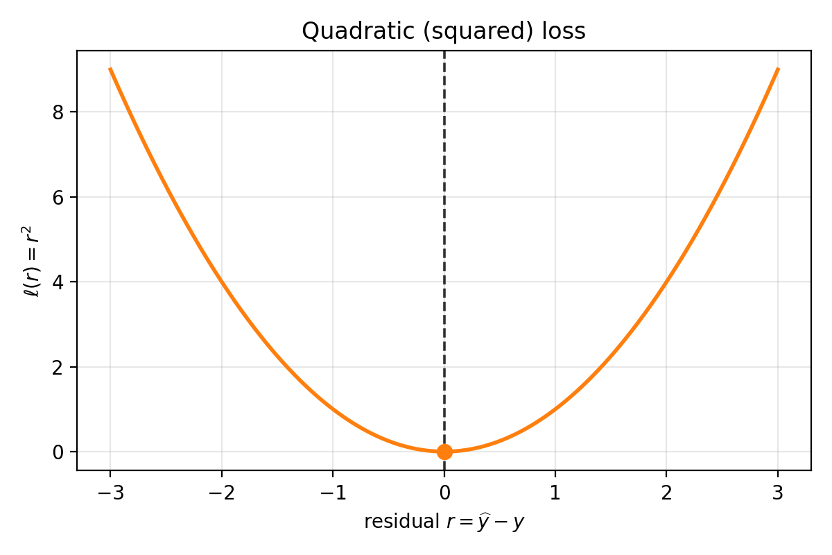
Quadratic loss as a function of residual $r=\widehat{y}-y$. It is symmetric around $r=0$ and grows quadratically as errors get larger.
Composing data, model, and loss:
\[L(w) = \frac{1}{n}\sum_{i=1}^n (w^T x_i - y_i)^2.\]This is exactly the pipeline Data $\rightarrow$ model $\rightarrow$ loss written as one objective in $w$. Minimize $L(w)$ and you have a predictor.
2.2 Sparsity: when you believe $w_\star$ has many zeros
What if you know more about $w_\star$? Suppose you suspect it is sparse – most coordinates are zero.
A natural first thought: constrain $w$ to have at most $s$ nonzero entries. Clean mathematical statement, but two immediate problems:
- The feasible set is nonconvex.
- We have not built the machinery for gradient-based methods with such constraints.
So we take a different approach.
2.2.1 $|w|_0$ regularization (the idea, and why it breaks gradient descent)
Define the $|w|_0$ “norm” (not actually a norm):
\[\|w\|_0 = \sum_{j=1}^d \mathbf{1}(w_j \neq 0).\]Then consider
\[\min_w \; L(w) + \lambda \|w\|_0.\]This encodes exactly what we want: penalize the number of nonzeros. Unfortunately, $|w|_0$ is combinatorial, what should the derivative of $\mathbf{1}(w_j \neq 0)$ be? PyTorch gradients are useless here.
Convex optimization gives us a way to relax this.
2.2.2 Convex envelope: replace $|x|_0$ by something convex
In 1D, $||x||_0$ is $0$ at $x=0$ and $1$ elsewhere. On $[-1,1]$, the function $\lvert x\rvert$ sits below $||x||_0$, and one can show it is the largest convex function lying below $|x|_0$ on that interval. This largest convex lower bound is called the convex envelope.
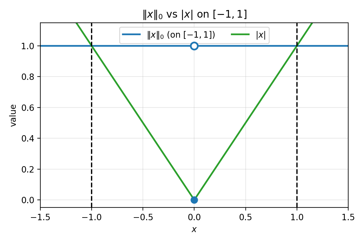
Figure 2.1: On $[-1,1]$, $|x|_0$ is $0$ at the origin and $1$ elsewhere. The function $\lvert x\rvert$ is the largest convex function that stays below $|x|_0$ on $[-1,1]$ (the convex envelope on that interval). The dashed lines mark $x=\pm 1$.
This motivates the $\ell_1$ regularizer.
2.2.3 $\ell_1$ regularization and the Lasso
Define $R_{\ell_1}(w) = ||w||_1 = \sum_{j=1}^d \lvert w_j\rvert$. The regularized objective becomes
\[\min_w \; \frac{1}{n}\sum_{i=1}^n (w^T x_i - y_i)^2 + \lambda \|w\|_1.\]This is the Lasso. It is convex, and as $\lambda$ increases the solution becomes sparser. In practice we do not know the right $\lambda$ in advance – we choose it by tuning against validation performance. That is important, but not the main point of this lecture.
2.3 Binary classification: $y$ is a label, not a number
Now let’s take a step back. Suppose the target is not a real number but a class label, with two classes $C_1$ and $C_2$.
We still use the same model: $m(x; w) = w^T x$. But the output is a real number, and $C_1$, $C_2$ are categorical. It does not make literal sense to demand $w^T x \approx C_1$, since $C_1$ could be a character string.
One workaround: encode $C_1 \mapsto 1$, $C_2 \mapsto -1$, and fit by squared loss. This can work, but it is not the natural loss for classification.
2.3.1 Logistic loss
Let $y \in \{-1, 1\}$ and define a score $a = w^T x$. The logistic loss is:
\[\ell(a, y) = \log\big(1+\exp(-ya)\big).\]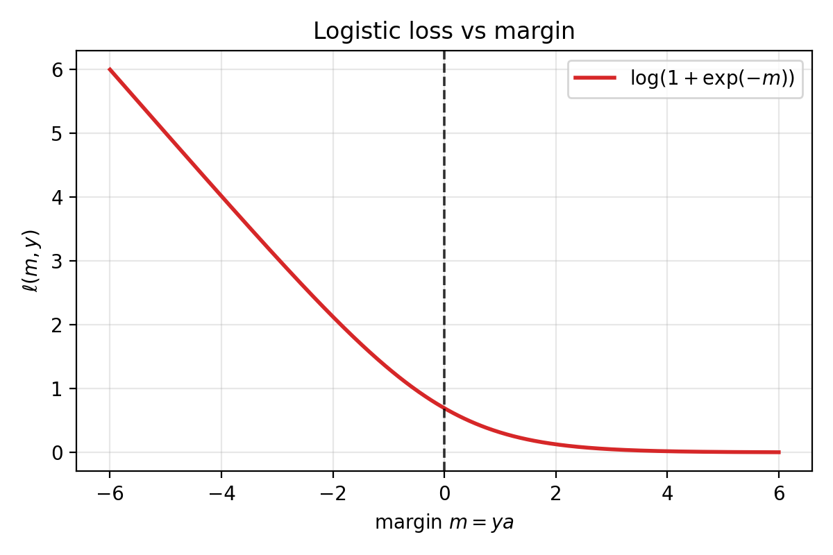
Logistic loss as a function of margin $m=ya$. Positive margin (correct sign) drives the loss toward $0$; negative margin incurs much larger loss.
When $y$ and $a$ have the same sign, $ya > 0$, so $\exp(-ya)$ is small and the loss is small. When they disagree, $ya < 0$ and the loss is large. Correct sign means low loss; wrong sign means high loss.
2.3.2 Probabilistic interpretation and MLE
Define the sigmoid $\operatorname{sigmoid}(t) = 1/(1+\exp(-t))$ and a conditional probability
\[P_w(y\mid x) = \operatorname{sigmoid}(y\, w^T x).\]We will take this quantity to be the model’s confidence that it assigned the correct label.
Now watch what happens when we take logs. Maximizing the log-likelihood of i.i.d. data means maximizing
\[\sum_{i=1}^n \log P_w(y_i \mid x_i).\]Equivalently, minimizing the negative log-likelihood:
\[-\frac{1}{n}\sum_{i=1}^n \log P_w(y_i \mid x_i).\]Using $\log(\operatorname{sigmoid}(t)) = -\log(1+\exp(-t))$, each term becomes
\[-\log P_w(y_i\mid x_i) = \log\big(1+\exp(-y_i w^T x_i)\big),\]which is exactly the logistic loss. The logistic loss is maximum likelihood estimation:
\[\arg\max_w \sum_{i=1}^n \log P_w(y_i\mid x_i) \;\Longleftrightarrow\; \arg\max_w \prod_{i=1}^n P_w(y_i\mid x_i),\]since log is monotone and we model the data as i.i.d. under $w$. You choose $w$ to maximize the likelihood of the observed labels under a simple probabilistic model.
2.3.3 Sparse logistic regression
Just like in regression, you can add an $\ell_1$ regularizer:
\[\min_w \; \frac{1}{n}\sum_{i=1}^n \log\big(1+\exp(-y_i w^T x_i)\big) + \lambda \|w\|_1.\]This encourages sparse classifiers.
2.4 PyTorch implementation
Everything above is easy to implement directly in PyTorch, without any torch.nn machinery. Store data in a matrix $X$ of shape (batch_size, d) with one sample per row, define a parameter vector $w$, and compute predictions as $Xw$.
import torch

torch.manual_seed(0)

n, d = 6, 4
X = torch.randn(n, d)

y_reg = torch.randn(n)                        # regression targets
y_cls = 2 * torch.randint(0, 2, (n,)) - 1     # binary labels in {+1, -1}

w = torch.randn(d)
logits = X @ w                                 # shape (n,)

# Squared loss
mse_loss = ((logits - y_reg) ** 2).mean()

# Logistic loss (torch.logaddexp for numerical stability)
logistic_loss = torch.logaddexp(torch.zeros_like(logits), -y_cls * logits).mean()

# L1 regularizer
l1 = w.abs().sum()
lam = 0.1

print("X.shape:", X.shape)                     # (6, 4)
print("logits.shape:", logits.shape)            # (6,)
print("mse_loss:", mse_loss.item())
print("logistic_loss:", logistic_loss.item())
print("mse + lam*l1:", (mse_loss + lam * l1).item())
print("logistic + lam*l1:", (logistic_loss + lam * l1).item())
That concludes the linear-model example. Next we move to richer models built by composing linear maps and nonlinearities – neural networks. In the next lecture, we will start on modern generative models (e.g., transformers), which are built from these same components.
3. Getting started with models in PyTorch
The model output shape and interpretation usually dictates the loss: scalar real output leads to regression losses (MSE), logits for classes lead to classification losses (logistic, cross-entropy). Generative models like transformers, which we cover next lecture, compose the same primitives we introduce here.
3.1 Models are compositions of simple maps
Most neural networks are built from three ingredients:
- linear maps (affine transformations)
- simple nonlinearities (applied componentwise)
- repetition / composition
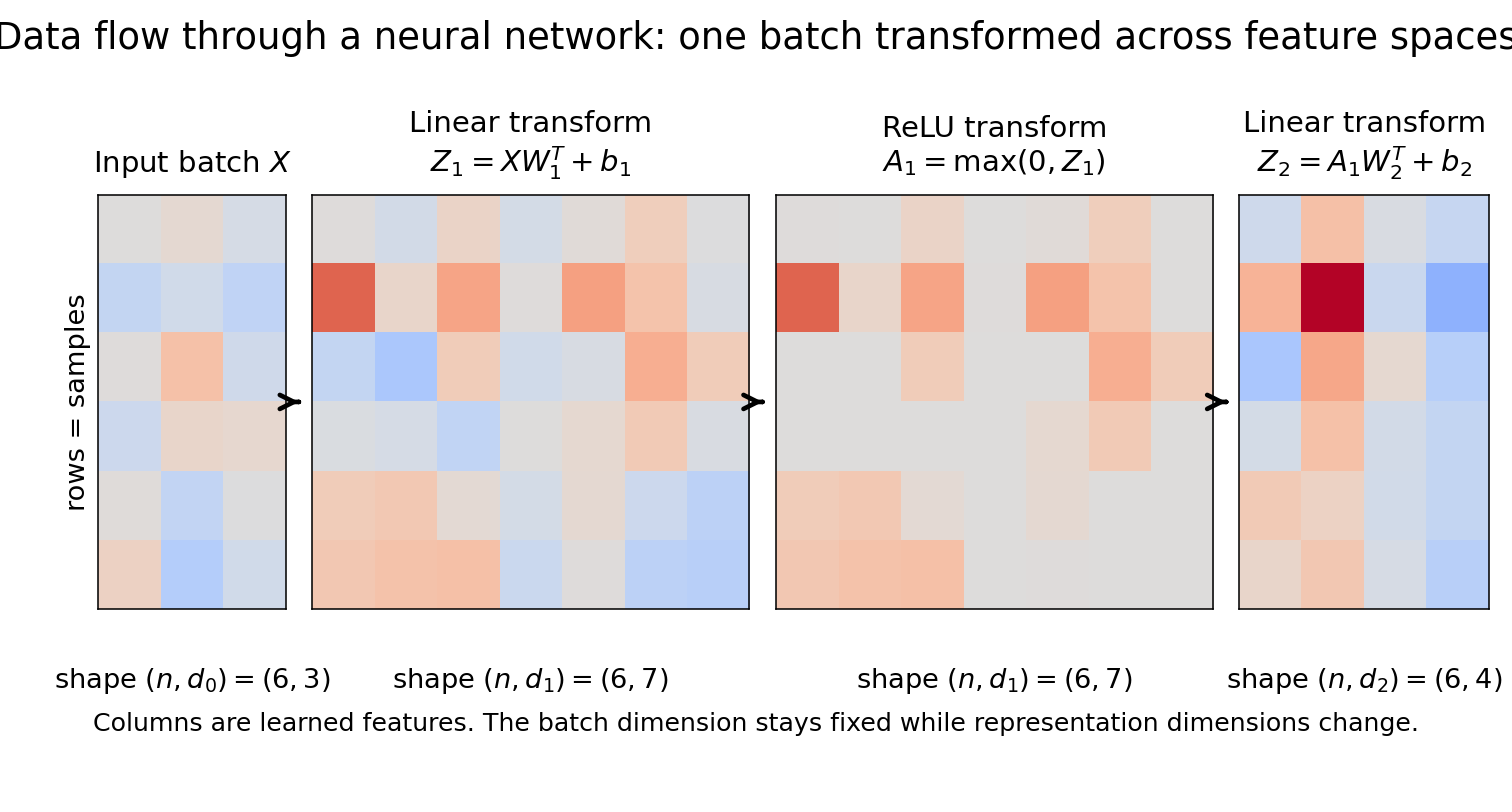
Figure 3.1: The same input batch flows through successive transformations: linear map $\rightarrow$ nonlinearity $\rightarrow$ linear map. The representation changes dimension across layers (from $(n,d_0)$ to $(n,d_1)$ to $(n,d_2)$), while the batch dimension $n$ is preserved.
Common nonlinearities you will see often:
- ReLU
- GELU
- SiLU (also called “Swish”)
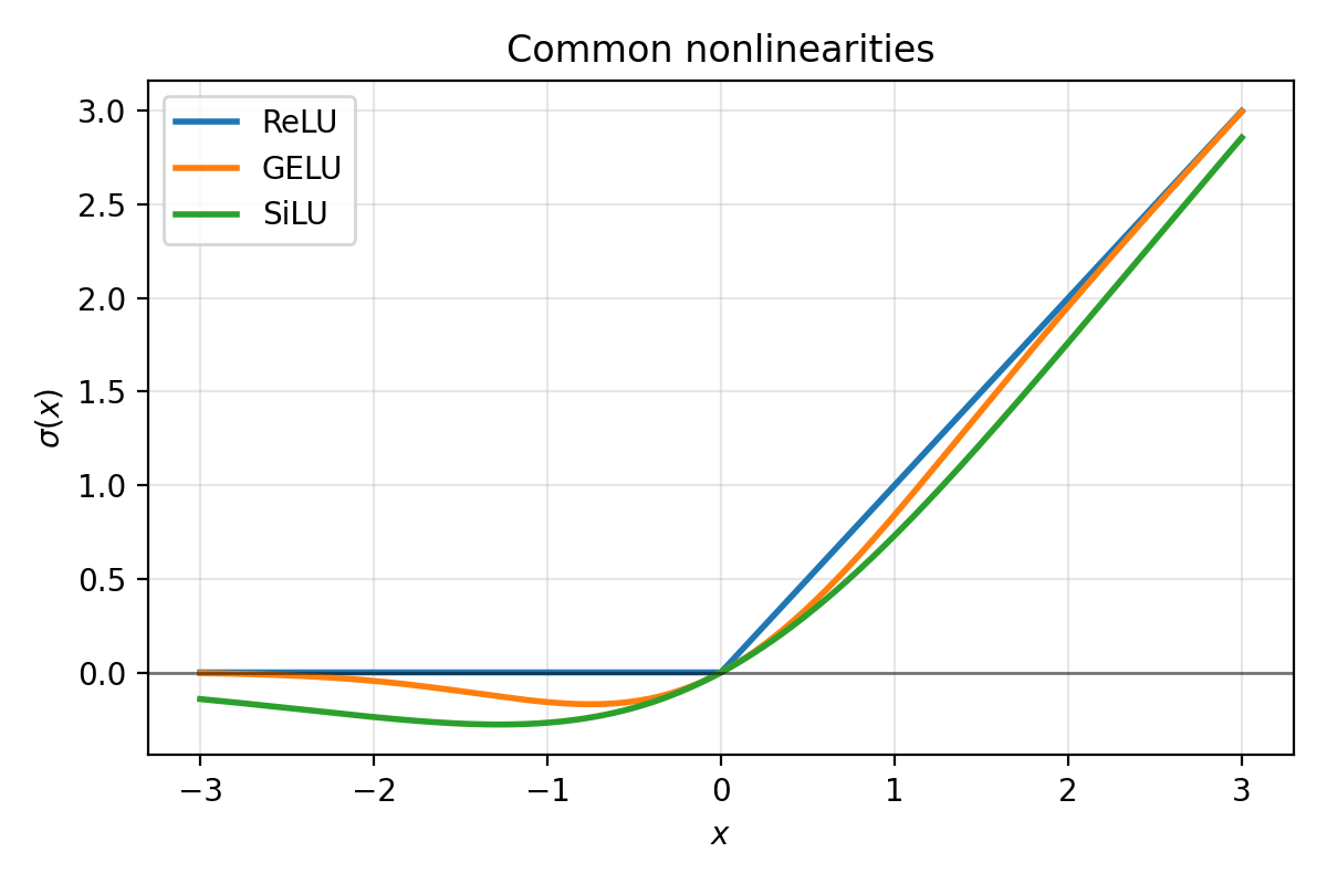
Figure 3.2: Typical activation functions. ReLU is exactly $0$ for negative inputs. GELU and SiLU are smooth and do not “hard clip” negative values.
3.2 PyTorch’s model toolbox (torch.nn)
PyTorch provides standard building blocks through torch.nn:
- linear maps:
torch.nn.Linear - convolutions:
torch.nn.Conv1d,torch.nn.Conv2d,torch.nn.Conv3d - containers:
torch.nn.Module
We chain layers and nonlinearities together inside a torch.nn.Module. Here is a preview:
class TwoLayerNet(torch.nn.Module):
    def __init__(self, d0, d1, d2):
        super().__init__()
        self.layer1 = torch.nn.Linear(d0, d1)
        self.layer2 = torch.nn.Linear(d1, d2)

    def forward(self, X):
        return self.layer2(torch.relu(self.layer1(X)))
We will explain Module in detail in Section 5. First we need to understand what the individual layers do and how shapes move through them.
3.3 Linear models and torch.nn.Linear
Goal: represent a linear model $m(x; w, b) = w^T x + b$ in PyTorch.
3.3.1 Batch-first convention and torch.nn.Linear
In PyTorch, a batch of vectors is stored as a matrix $X$ of shape (batch_size, input_features), with each row being one sample:
This convention is not optional. Internalize it early.
A torch.nn.Linear(d, k) layer maps (n, d) to (n, k):
m = torch.nn.Linear(in_features=d, out_features=k, bias=True)
3.3.2 Weight storage and the transpose
PyTorch stores m.weight with shape (k, d) and m.bias with shape (k,). The forward computation is:
where $X$ is $(n,d)$, $W^T$ is $(d,k)$, and $b$ broadcasts across the batch. The output is $(n,k)$.
Row $j$ of m.weight is the weight vector for output coordinate $j$ – one row per “neuron.”
Why the transpose? In math, we think of transforming a column vector $y = Wx + b$. PyTorch stores data as rows and multiplies on the right, so the same map becomes $Y = XW^T + b$. The transpose is bookkeeping caused by “samples are rows.” This batch-first convention matches the data-table convention (rows = samples, columns = features), generalizes cleanly (Linear acts on the last dimension of any tensor (*, d) -> (*, k)), and keeps each sample’s feature vector contiguous in row-major memory; this makes it fast to retrieve a sample’s features as a contiguous vector.
The output dimension $k$ controls what the layer does:
- $k = 1$: a scalar classifier/regressor.
m.weightis $(1,d)$ – one weight vector. Output is $(n,1)$, exactly $w^T x_i + b$ in batch form. - $k > 1$: $k$ different weight vectors, one per output coordinate. Output is $(n,k)$. For regression, these are $k$ real targets; for classification, they are $k$ logits.
3.3.3 Bias shifts the decision boundary
Without bias, the decision boundary $w^T x = 0$ must pass through the origin. With bias, $w^T x + b = 0$ can shift freely. If your data is not centered at the origin, the no-bias model is unnecessarily restricted.
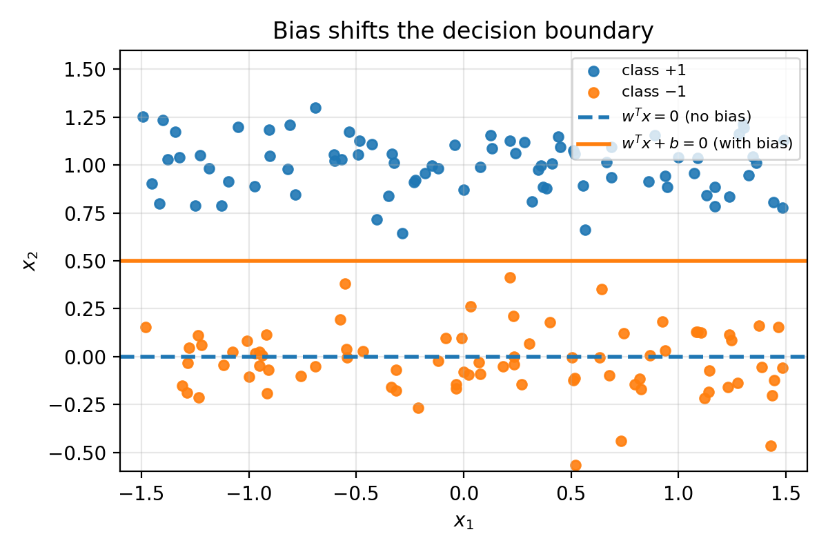
Figure 3.3: In 2D, $w^T x = 0$ is always a line through the origin. Adding a bias shifts the line.
3.4 Composing linear layers into a neural network
This is the first real step toward deep learning. A single Linear layer is one affine map. A neural network composes many such layers with nonlinearities in between:
- $A_0 = X$ has shape $(n, d_0)$.
- Pre-activation: $Z_\ell = A_{\ell-1} W_\ell^T + b_\ell$ with shape $(n, d_\ell)$.
- Activation: $A_\ell = \sigma(Z_\ell)$ with shape $(n, d_\ell)$.
The batch dimension $n$ is always preserved. The feature dimension changes at each layer: $d_0 \to d_1 \to \cdots \to d_L$.
3.4.1 PyTorch code: a 2-layer network as a plain function
import torch

torch.manual_seed(0)

n = 4      # batch size
d0 = 5     # input dimension
d1 = 10    # hidden dimension
d2 = 3     # output dimension

X = torch.randn(n, d0)

layer1 = torch.nn.Linear(d0, d1, bias=True)
layer2 = torch.nn.Linear(d1, d2, bias=True)

def m(X):
    Z1 = layer1(X)       # Z1 = X W1^T + b1
    A1 = torch.relu(Z1)
    Z2 = layer2(A1)       # Z2 = A1 W2^T + b2
    return Z2

Z1 = layer1(X)
A1 = torch.relu(Z1)
Z2 = layer2(A1)

print("X.shape:", X.shape)                # (4, 5)
print("Z1.shape:", Z1.shape)              # (4, 10)
print("A1.shape:", A1.shape)              # (4, 10)
print("Z2.shape:", Z2.shape)              # (4, 3)

print("layer1.weight.shape:", layer1.weight.shape)  # (10, 5) = (d1, d0)
print("layer2.weight.shape:", layer2.weight.shape)  # (3, 10) = (d2, d1)

# Autograd sanity check: compute a dummy loss, call backward
Y = torch.randn(n, d2)
loss = ((Z2 - Y) ** 2).mean()
loss.backward()

print("loss:", loss.item())
print("||grad layer1.weight||:", layer1.weight.grad.norm().item())
print("||grad layer2.weight||:", layer2.weight.grad.norm().item())
A torch.nn.Linear layer is already a linear map, but it treats every input coordinate independently. What if the input has spatial structure – pixels in an image, samples in a time series? That is what convolution layers are for.
4. Convolution layers as linear maps with weight sharing
4.1 Convolutions as pattern detectors reused across space
A Linear layer assigns one weight per input coordinate. But signals and images have spatial structure: the same local pattern (an edge, a pulse, a corner) can appear in many locations. We want to detect it anywhere without learning separate weights for every position.
The idea: learn a small set of weights – a kernel – and slide it across the input, taking a dot product at each location. This is weight sharing: one small kernel parameterizes a large linear map.
A 1D conv filter is a sliding dot product with a small pattern, producing a “match score” at each location. Large positive response means “this patch looks like the pattern”; negative means “looks like the opposite.”
4.2 1D illustration: signal + kernel + response
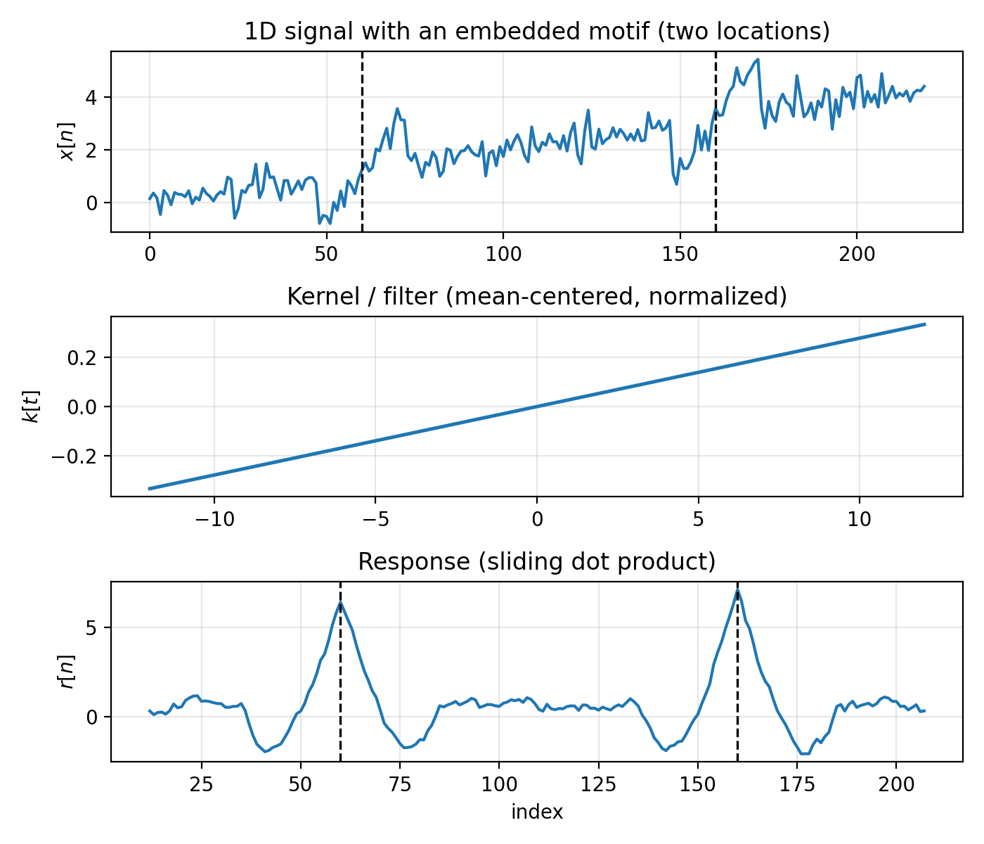
Figure 4.1: Top: a 1D signal $x[n]$ with a short motif embedded at two locations (dashed vertical lines mark the motif centers). Middle: the kernel $k[t]$ (mean-centered, normalized). Bottom: the response $r[n]$ produced by sliding $k$ over $x$ and taking dot products. Peaks occur near the embedded motifs.
Key parameters:
- Kernel (filter): a short trainable template slid across the signal. In Figure 4.1, the middle plot is this template.
- Input channels (
C_in): number of parallel signal streams at each index. Figure 4.1 is single-channel. - Output channels (
C_out): number of detectors you learn. Each produces its own response signal. - Stride: how many indices the kernel shifts each step.
stride = 1checks every position;stride = 2skips every other. - Padding: zeros added at boundaries so edge locations are treated more like interior ones.
PyTorch syntax:
conv1d = torch.nn.Conv1d(in_channels=C_in, out_channels=C_out, kernel_size=k, stride=1, padding=0, bias=True)
- input shape:
(batch_size, C_in, L) - weight shape:
(C_out, C_in, k) - output shape:
(batch_size, C_out, L_out)
For each output channel $j$:
\[r_j(n) = \sum_{c=1}^{C_\text{in}} \langle \text{local patch from channel } c,\; k_{j,c}\rangle + b_j.\]The layer combines information across input channels by summing channel-wise responses. If C_out = 2, you get two separate response signals $r_1(n)$ and $r_2(n)$; they are not summed together.
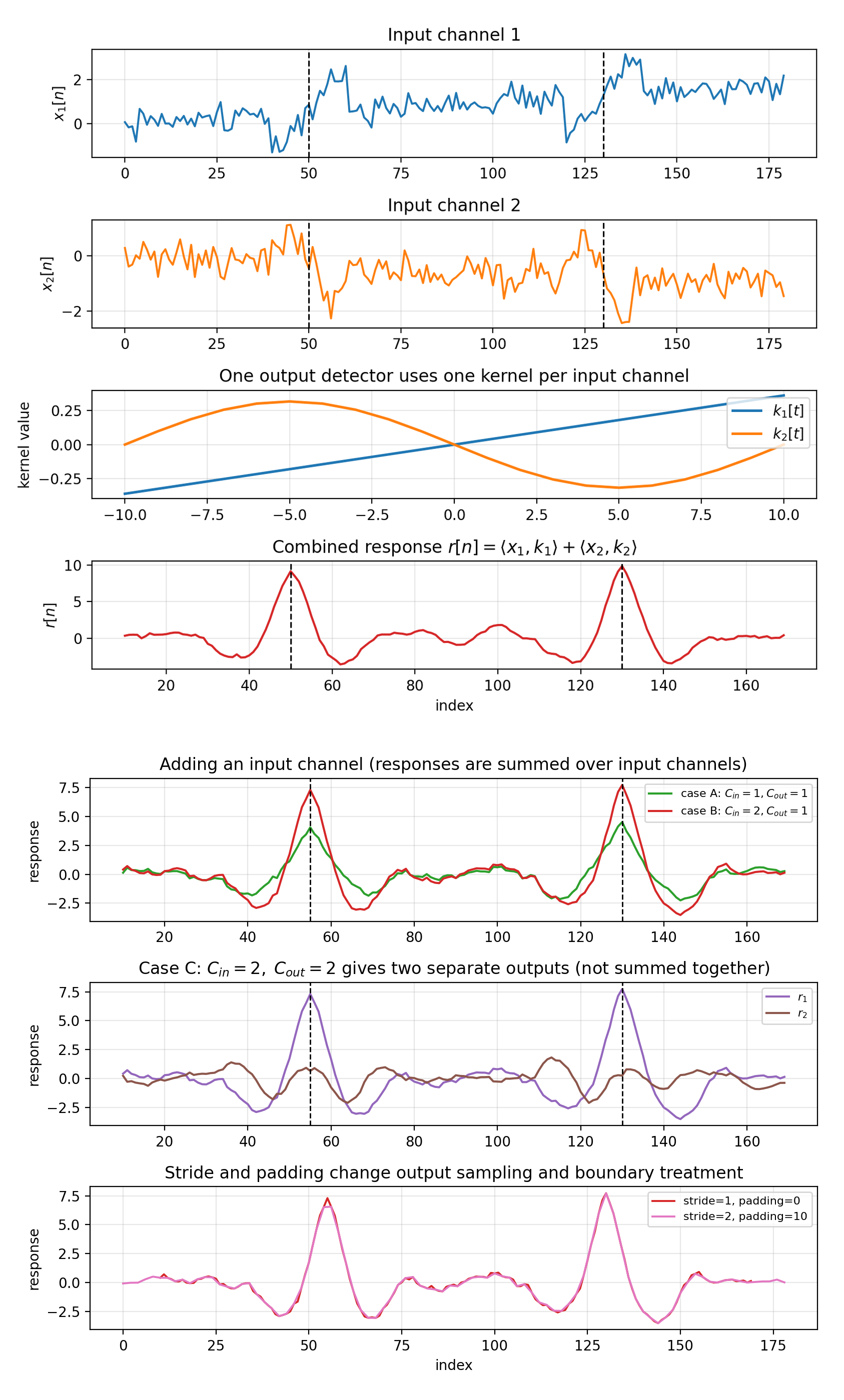
Figure 4.1b: Two views of the same synthetic setup. Top panel: one detector with C_in=2, C_out=1, where the response is the channel-summed signal $r(n)=\langle x_1,k_1\rangle+\langle x_2,k_2\rangle$. Bottom panel (three rows) reuses the same inputs from the top panel: row 1 (“adding an input channel”) compares C_in=1 -> C_out=1 against C_in=2 -> C_out=1; row 2 shows C_in=2 -> C_out=2 (two separate outputs); row 3 changes stride/padding for the same detector to show output resampling and boundary effects.
4.3 Matrix view: convolution as a Toeplitz linear map
If you store 1D signals as row vectors with a batch dimension, $X$ has shape (batch_size, N). Convolution by a fixed kernel is a linear map on the right:
where $K$ is a Toeplitz (banded) matrix whose rows are shifted copies of the same kernel weights. The matrix is large, but completely determined by a small kernel $k$ – that is the weight sharing. The transpose is the same bookkeeping as torch.nn.Linear: one output feature per row of $K$, multiply on the right to preserve batch-first layout.
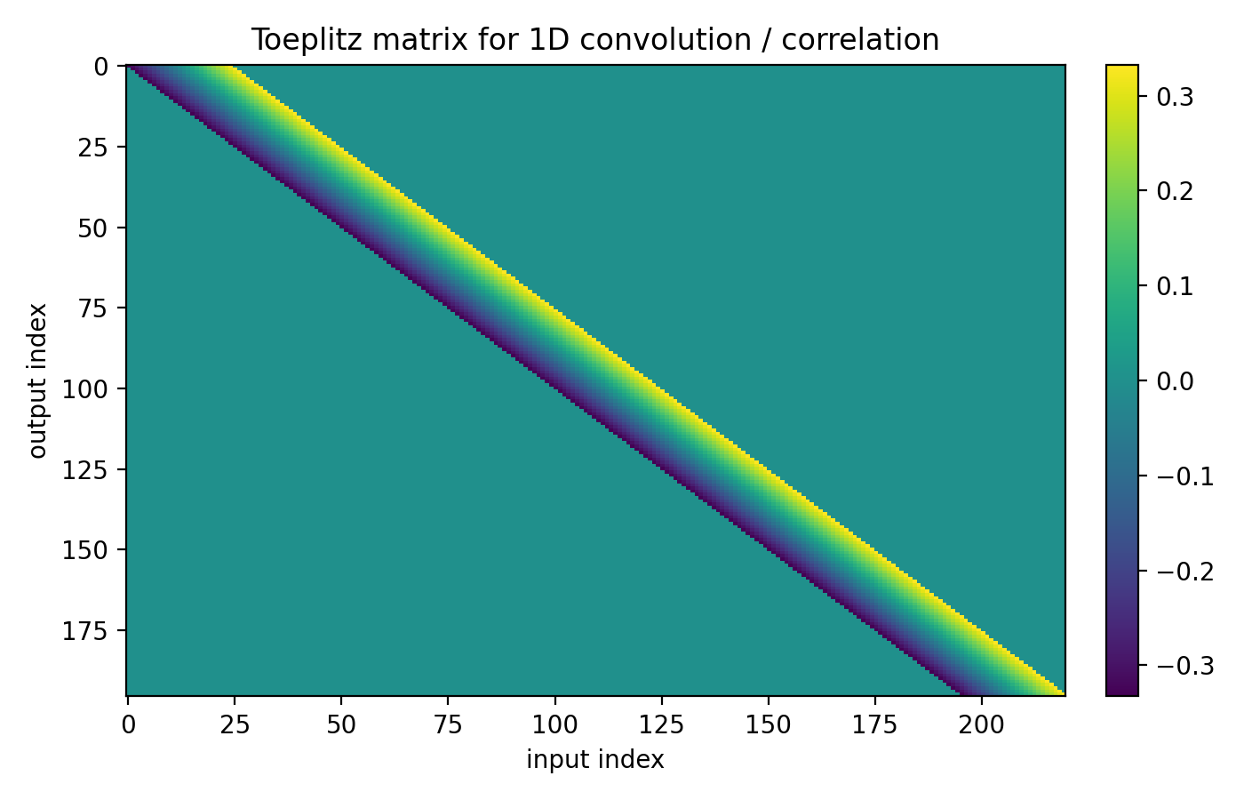
Figure 4.2: A Toeplitz matrix $K$ encoding a 1D sliding dot product. Each row is a shifted copy of the same kernel weights. The linear map is huge, but parameterized by a short vector.
Shape summary:
- Single-channel: signal length $N$, kernel length $m$ with $m \ll N$.
- Multi-channel: input has $C_\text{in}$ channels, weights have shape
(C_out, C_in, m), output has $C_\text{out}$ channels.
The weights live in “local patch dimensions” (and channel depth), not in the full signal length.
4.4 2D illustration: image + kernel + feature map
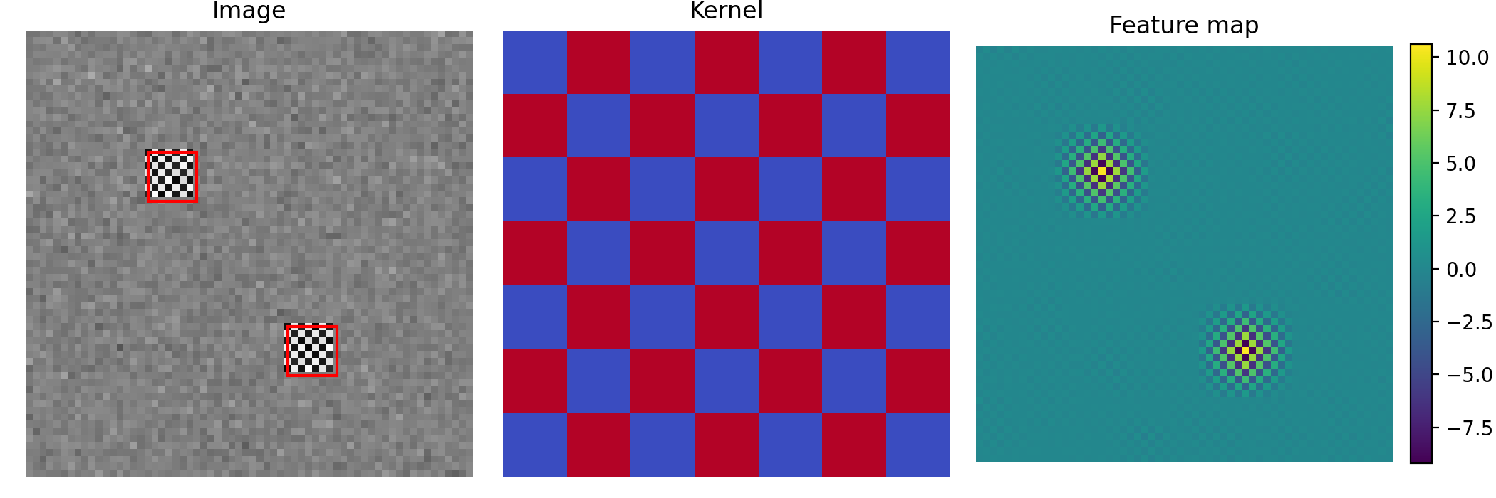
Figure 4.3: Left: a synthetic image with a small motif repeated at two locations (red boxes). Middle: a small kernel. Right: the feature map produced by sliding the kernel over the image. Bright spots indicate matches.
PyTorch syntax:
conv2d = torch.nn.Conv2d(in_channels=C_in, out_channels=C_out, kernel_size=(kH, kW), stride=1, padding=0, bias=True)
Each output channel is one learned 2D detector. At each spatial location $(u,v)$, detector $j$ reads a local patch from every input channel, computes channel-wise dot products, sums them, and adds a bias:
\[r_j(u,v) = \sum_{c=1}^{C_\text{in}} \langle \text{local 2D patch from channel } c,\; K_{j,c}\rangle + b_j.\]Shape summary (2D):
- input:
(batch_size, C_in, H, W) - weights:
(C_out, C_in, kH, kW) - output:
(batch_size, C_out, H_out, W_out)
If you flatten each image into a row vector, 2D convolution is again $R = X K^T$ where $K$ is sparse block-Toeplitz. Same moral: huge implied linear map, small local kernel.
4.5 3D convolution
3D convolution extends the idea to three spatial axes:
- Volumetric data (MRI, CT scans as voxel grids): the kernel slides over depth $\times$ height $\times$ width to detect 3D features like lesions or anatomical landmarks.
- Video (frames stacked along time): the kernel slides over time $\times$ height $\times$ width to detect spatiotemporal patterns like a moving edge or gesture.
conv3d = torch.nn.Conv3d(in_channels=C_in, out_channels=C_out, kernel_size=(kD, kH, kW), stride=1, padding=0, bias=True)
Shape summary (3D):
- input:
(batch_size, C_in, D, H, W) - weights:
(C_out, C_in, kD, kH, kW) - output:
(batch_size, C_out, D_out, H_out, W_out)
4.6 Summary: 1D vs 2D vs 3D
The “dimension” is the space you slide over:
- 1D: one axis (time, sequence index)
- 2D: a grid (height $\times$ width)
- 3D: a volume (depth/time $\times$ height $\times$ width)
In all cases, channels work the same way: each detector sums channel-wise local dot products over $C_\text{in}$ and produces one output channel.
4.7 Pooling: turning feature maps into prediction-ready vectors
Convolutional layers return tensors with spatial structure, e.g. (B, C_out, H, W) in 2D. Prediction heads need one vector per sample, so we reduce spatial dimensions while keeping channel information.
Local pooling. Slide a $k \times k$ window with stride $s$ over each channel map $M \in \mathbb{R}^{H \times W}$. At each window position $(u,v)$, average pooling returns the mean of the $k^2$ values in that window; max pooling returns the maximum:
\[\mathrm{AvgPool}_{k,s}(M)_{u,v} = \operatorname{mean}(\text{window at } u,v), \qquad \mathrm{MaxPool}_{k,s}(M)_{u,v} = \max(\text{window at } u,v).\]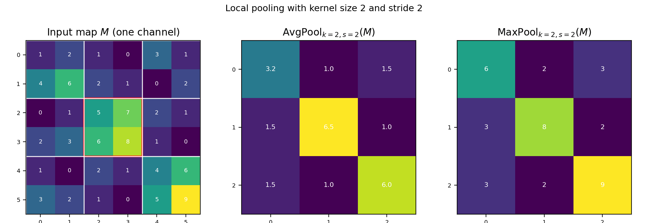
Figure 4.4a: A single-channel map $M$ with window size k=2, stride s=2. White grid lines mark pooling windows. Middle: average pooling output. Right: max pooling output.
Global pooling (GP). Reduce each channel map to a single number by averaging or taking the max over all spatial positions. If $P$ has shape $(B, C_\text{out}, H’, W’)$, then $g = \mathrm{GP}(P)$ has shape $(B, C_\text{out})$ – one scalar per channel per sample.
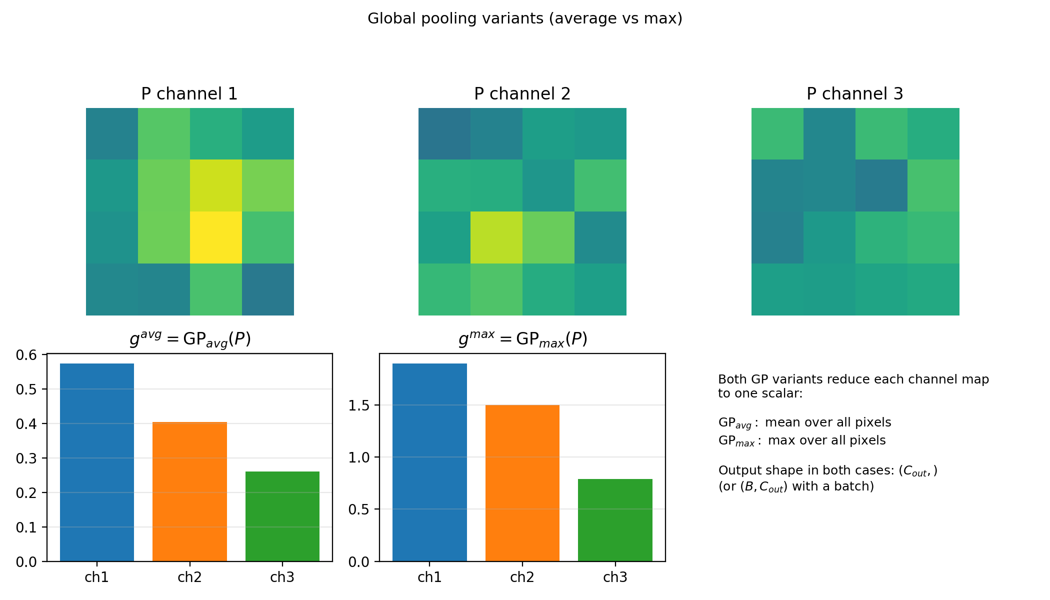
Figure 4.4b: Global average and global max pooling both return one scalar per channel (same shape). They differ only in reduction rule (mean vs max over the full spatial map).
The full prediction pipeline:
\[P = \mathrm{Pool}_{k,s}(A),\qquad g = \mathrm{GP}(P),\qquad z = g\, W_{\text{head}}^T + b_{\text{head}}.\]Here $z$ has shape $(B, \text{num_classes})$.
PyTorch syntax:
pool_local = torch.nn.AvgPool2d(kernel_size=2, stride=2)  # or MaxPool2d
P = pool_local(A)                                          # (B, C_out, H', W')

g = torch.nn.functional.adaptive_avg_pool2d(P, output_size=1).flatten(1)  # (B, C_out)
head = torch.nn.Linear(C_out, num_classes)
logits = head(g)                                           # (B, num_classes)
(AvgPool1d/3d, MaxPool1d/3d, and adaptive_avg_pool1d/3d are the 1D and 3D analogs.)
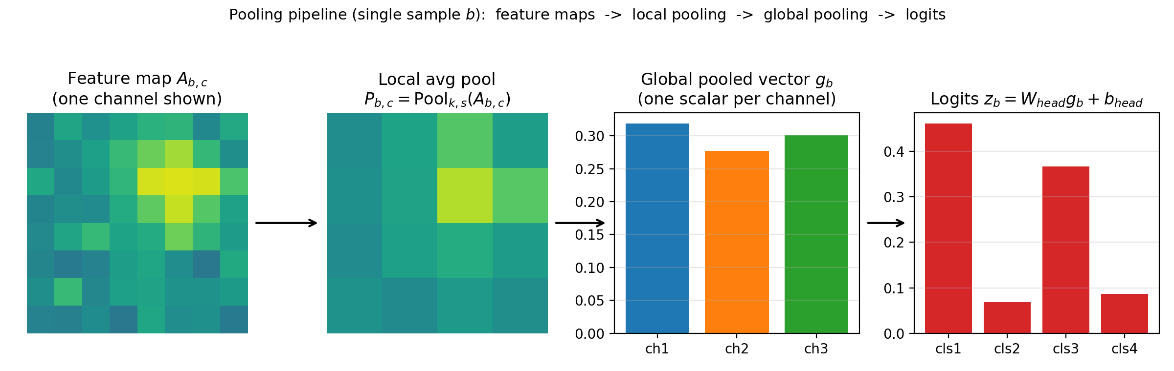
Figure 4.4c: Pipeline view for one sample. Pool feature maps, collapse spatial dimensions with GP, then apply a linear head.
4.8 A small CNN implementation
Batch-first still holds, but conv layers expect channels-first tensors: the channel axis comes right after the batch axis, before any spatial dimensions.
import torch

torch.manual_seed(0)

batch_size, C_in, H, W = 2, 3, 32, 32
X = torch.randn(batch_size, C_in, H, W)

C_hidden, C_out = 8, 16
conv1 = torch.nn.Conv2d(C_in, C_hidden, kernel_size=3, stride=1, padding=1, bias=True)
conv2 = torch.nn.Conv2d(C_hidden, C_out, kernel_size=3, stride=1, padding=1, bias=True)

Z1 = conv1(X)
A1 = torch.relu(Z1)
Z2 = conv2(A1)

print("X.shape:", X.shape)    # (2, 3, 32, 32)
print("Z1.shape:", Z1.shape)  # (2, 8, 32, 32)
print("Z2.shape:", Z2.shape)  # (2, 16, 32, 32)

print("conv1.weight.shape:", conv1.weight.shape)  # (8, 3, 3, 3) = (C_out, C_in, kH, kW)
print("conv2.weight.shape:", conv2.weight.shape)  # (16, 8, 3, 3)

# Bridge to classification: pool away spatial dims, then linear head
pooled = Z2.mean(dim=(2, 3))       # (2, 16)
num_classes = 5
head = torch.nn.Linear(C_out, num_classes)
logits = head(pooled)
print("logits.shape:", logits.shape)  # (2, 5)
5. Introducing torch.nn.Module (the standard model container)
A Module bundles learnable parameters and forward computation into one object. The recipe:
- Define a class inheriting from
torch.nn.Module. - In
__init__: callsuper().__init__(), create layers as attributes. - In
forward(self, X): write the computation, return the output. - Call the object like a function:
model(X).
5.1 A minimal Module
import torch

class TwoLayerNet(torch.nn.Module):
    def __init__(self, d0, d1, d2):
        super().__init__()
        self.layer1 = torch.nn.Linear(d0, d1, bias=True)
        self.layer2 = torch.nn.Linear(d1, d2, bias=True)

    def forward(self, X):
        Z1 = self.layer1(X)
        A1 = torch.relu(Z1)
        Z2 = self.layer2(A1)
        return Z2

torch.manual_seed(0)

n, d0, d1, d2 = 4, 5, 10, 3
X = torch.randn(n, d0)

model = TwoLayerNet(d0, d1, d2)
out = model(X)

print("out.shape:", out.shape)                  # (4, 3)
print("number of parameter tensors:", len(list(model.parameters())))  # 4
for p in model.parameters():
    print("  param shape:", tuple(p.shape))
Define layers in __init__, wire them in forward, call the model like a function. PyTorch uses forward to build a computation graph for automatic gradients.
5.2 Why Module over a plain function
A plain function computes the same output, but Module gives you infrastructure for free:
- Parameter registration –
model.parameters()collects every learnable tensor automatically. - Saving/loading –
model.state_dict()serializes all parameters;load_state_dict()restores them. - Device management –
model.to(device)moves every parameter to CPU/GPU together. - Train/eval modes –
model.train()/model.eval()toggle layers like dropout and batchnorm. - Composition and introspection – Modules nest inside other Modules;
named_parameters()andnamed_modules()make debugging systematic.
5.3 A convolutional Module
import torch

class SmallCNN(torch.nn.Module):
    def __init__(self, C_in, C_hidden, C_out, num_classes):
        super().__init__()
        self.conv1 = torch.nn.Conv2d(C_in, C_hidden, kernel_size=3, padding=1, bias=True)
        self.conv2 = torch.nn.Conv2d(C_hidden, C_out, kernel_size=3, padding=1, bias=True)
        self.head = torch.nn.Linear(C_out, num_classes, bias=True)

    def forward(self, X):
        A1 = torch.relu(self.conv1(X))
        A2 = torch.relu(self.conv2(A1))
        pooled = A2.mean(dim=(2, 3))
        return self.head(pooled)

torch.manual_seed(0)

X = torch.randn(2, 3, 32, 32)
model = SmallCNN(C_in=3, C_hidden=8, C_out=16, num_classes=5)
logits = model(X)

print("logits.shape:", logits.shape)            # (2, 5)
print("num parameter tensors:", len(list(model.parameters())))  # 7
print("state_dict keys:", list(model.state_dict().keys())[:5])
6. Putting it together: the training loop
We introduced squared loss and logistic loss in Section 2. Now that we have Module containers, here is how all the pieces fit into a training step.
6.1 The training skeleton
Whether you are training a regression model or a classifier, the loop is the same:
- Start with a mini-batch
(X, y). - Forward pass:
logits = model(X). - Evaluate a scalar loss:
loss = loss_fn(logits, y). - Backward pass:
loss.backward()– computes gradients of the loss with respect to every parameter. - Update parameters (via an optimizer or manual step).
- Zero gradients before the next batch.
Logits are the raw model outputs before any final sigmoid or softmax. The loss function handles the conversion internally.
6.2 Which loss for which task
Section 2 derived the losses from first principles. Here is the summary with PyTorch function names:
| Task | Loss | PyTorch |
|---|---|---|
| Regression | $\frac{1}{n}\sum(\widehat{y}_i - y_i)^2$ | F.mse_loss(logits, y) |
| Binary classification | $\log(1+\exp(-y\cdot a))$ | F.binary_cross_entropy_with_logits(logits, y) |
| Multi-class classification | cross-entropy on logits | F.cross_entropy(logits, y) (expects integer labels) |
Important: cross_entropy takes logits directly. Do not apply softmax first.
6.3 Computing a loss and inspecting gradients
After loss.backward(), every parameter tensor has a .grad field storing its gradient.
import torch
import torch.nn.functional as F

torch.manual_seed(0)

class TwoLayerNet(torch.nn.Module):
    def __init__(self, d0, d1, d2):
        super().__init__()
        self.layer1 = torch.nn.Linear(d0, d1, bias=True)
        self.layer2 = torch.nn.Linear(d1, d2, bias=True)

    def forward(self, X):
        return self.layer2(torch.relu(self.layer1(X)))

batch_size, d0, d1, num_classes = 8, 5, 12, 4
X = torch.randn(batch_size, d0)
y = torch.randint(0, num_classes, (batch_size,))

model = TwoLayerNet(d0, d1, num_classes)
logits = model(X)

loss_value = F.cross_entropy(logits, y)
print("loss:", loss_value.item())

loss_value.backward()

for name, p in model.named_parameters():
    print(f"  {name}: param {tuple(p.shape)}, grad norm {p.grad.norm().item():.4f}")
6.4 Zeroing gradients
Gradients accumulate by default in PyTorch – calling backward() twice without resetting adds to the existing .grad. The fix: zero gradients once per batch, either with model.zero_grad() or (more commonly) optimizer.zero_grad().
7. Conclusion
We now have the full formulation toolkit: data and models compose into a loss, regularizers encode prior knowledge, and backward() produces the gradients you need for training. Linear and convolutional layers are the two fundamental building blocks; torch.nn.Module is how you package them. Next lecture: modern generative models (e.g., transformers) built from these same pieces.