Adagrad, Adam, and AdamW: Cheat Sheet / Slides

Slide 1: The Problem w/ SGD

• Core Issue: Standard SGD uses a single learning rate ($\alpha$) for all parameters.
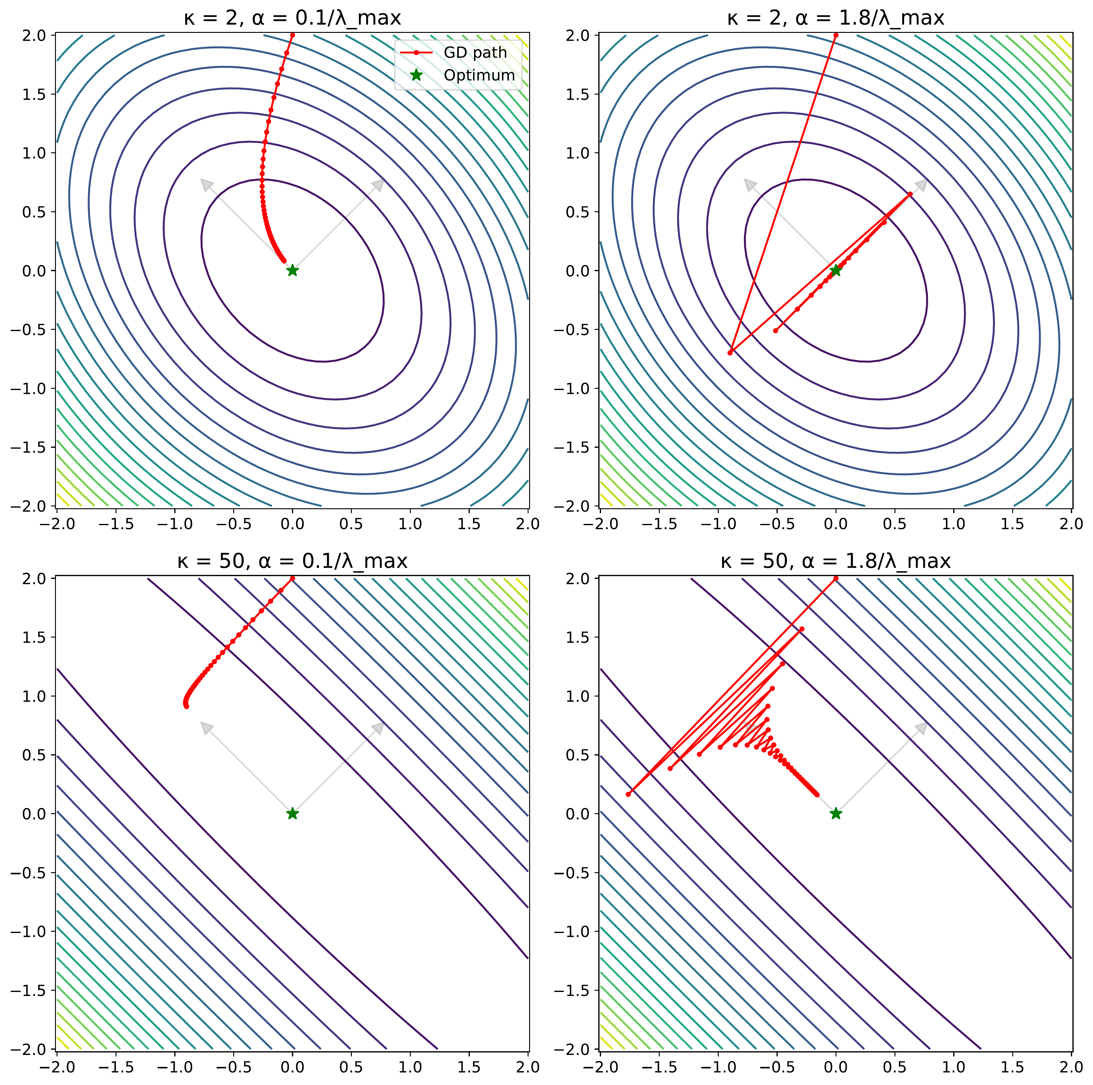
• Problem 1: Feature Scaling Sensitivity: Features with different scales -> loss landscape has elongated valleys/ravines.
• Problem 2: Ill-Conditioning: Measured by condition number $\kappa = \lambda_{max}(H) / \lambda_{min}(H)$. Large $\kappa$ means difficult optimization.
  • Example: $L(w) = \frac{1}{2}(h_1 w_1^2 + h_2 w_2^2)$ with $h_1 \gg h_2$.
• SGD Trade-off: Need small $\alpha$ for stability in steep directions (large curvature, $h_1$), but this means very slow progress in flat directions (small curvature, $h_2$). Convergence rate can be like $(1 - h_2/h_1)^k$.
• Visual: (Conceptually) A contour plot showing an elongated ellipse, with SGD oscillating across the narrow axis and moving slowly along the long axis.

Slide 2: The Adaptive Idea

• Core Idea: Give each parameter $w_i$ its own adaptive learning rate.
• Mechanism: Scale the learning rate inversely proportional to some measure of historical gradient magnitudes for that parameter.
  • Large historical gradients -> smaller effective LR.
  • Small historical gradients -> larger effective LR.
• Goal: Address scaling sensitivity and ill-conditioning automatically.
• Lineage: Adagrad (accumulate squares) -> RMSProp (EMA of squares) -> Adam (RMSProp + Momentum + Bias Correction) -> AdamW (Adam + Decoupled Weight Decay).

Slide 3: Adagrad (Duchi et al., 2011)

• Goal: Adapt LR per parameter based on sum of historical squared gradients.
• Gradient: $g_t = \nabla \ell(w_{t-1}, z_t)$
• Accumulator: $G_{t,ii} = \sum_{j=1}^{t} g_{j,i}^2$ (sum of squares for param $i$ up to time $t$)
• Update Rule (per parameter $i$): \(w_{t,i} = w_{t-1,i} - \frac{\alpha}{\sqrt{G_{t,ii} + \epsilon}} \cdot g_{t,i}\)
  • $\alpha$: Global learning rate.
  • $\epsilon$: Small constant for numerical stability (e.g., $10^{-8}$).
• Pros: Good for sparse gradients (infrequent updates get larger LR when they occur). Eliminates manual per-param LR tuning.
• Cons: $G_{t,ii}$ only increases. Effective LR monotonically decreases -> can eventually become too small, stalling learning.

Slide 4: Adam (Kingma & Ba, 2015) - Intro

• Name: Adaptive Moment Estimation.
• Goal: Combine adaptive learning rates (like RMSProp, using EMAs instead of sums) with momentum.
• Key Idea: Track Exponential Moving Averages (EMAs) of:
  1. First Moment (Mean): $m_t$
  2. Second Moment (Uncentered Variance): $v_t$

Slide 5: Adam - Mechanics: Moment Updates

• Gradient: $g_t = \nabla \ell(w_{t-1})$
• First Moment Estimate (Momentum): \(m_t = \beta_1 m_{t-1} + (1 - \beta_1) g_t\)
  • $\beta_1$: Exponential decay rate for the first moment (e.g., 0.9).
• Second Moment Estimate (Uncentered Variance): \(v_t = \beta_2 v_{t-1} + (1 - \beta_2) g_t^2 \quad \text{(element-wise square)}\)
  • $\beta_2$: Exponential decay rate for the second moment (e.g., 0.999).
• Issue: $m_t$ and $v_t$ are initialized at 0 and are biased towards zero, especially early in training when $t$ is small.

Slide 6: Adam - Mechanics: Bias Correction

• Why? EMAs initialized at zero underestimate moments early on.
  • Consider $m_0 = 0$ and constant gradient $g$. Then $m_t = (1 - \beta_1^t) g$. The estimate is scaled by $(1 - \beta_1^t)$, which is small for small $t$. Similar logic applies to $v_t$.
• Bias-Corrected First Moment: \(\hat{m}_t = \frac{m_t}{1 - \beta_1^t}\)
• Bias-Corrected Second Moment: \(\hat{v}_t = \frac{v_t}{1 - \beta_2^t}\)
• Effect: Correction factors $(1 - \beta_1^t)$ and $(1 - \beta_2^t)$ start small and approach 1 as $t \to \infty$. This counteracts the initial bias.

Slide 7: Adam - Update Rule & Interpretation

• Full Update Rule: \(w_t = w_{t-1} - \alpha \frac{\hat{m}_t}{\sqrt{\hat{v}_t} + \epsilon}\)
  • $\alpha$: Step size (learning rate, e.g., 0.001).
  • $\epsilon$: Small constant for numerical stability (e.g., $10^{-8}$).
  • Operations ($\sqrt{\cdot}$, division) are element-wise.
• Interpretation:
  • $\frac{\alpha}{\sqrt{\hat{v}_t} + \epsilon}$: Adaptive learning rate per parameter. Scales inversely with root mean square of recent gradients.
  • $\hat{m}_t$: Momentum term, provides smoothed gradient direction.
• Hyperparameters: $\alpha, \beta_1, \beta_2, \epsilon$. Defaults: $\beta_1=0.9, \beta_2=0.999, \epsilon=10^{-8}$. Tuning matters.

Slide 8: AdamW (Loshchilov & Hutter, 2019)

• Problem: Standard L2 regularization ($\frac{\lambda}{2}|w|_2^2$) interacts poorly with Adam’s adaptive scaling.
  • In SGD, L2 reg $\iff$ Weight Decay: $w_t = (1 - \alpha\lambda)w_{t-1} - \alpha\nabla \ell$.
  • In Adam, the gradient term $g_t = \nabla \ell + \lambda w_{t-1}$ gets included in $m_t$ and $v_t$, so the effective weight decay depends on $\sqrt{\hat{v}_t}$, making it inconsistent across parameters.
• AdamW Solution: Decouple weight decay from the adaptive gradient update.
• AdamW Update Rule:
  1. Apply weight decay directly: \(w_{t-1}'= (1 - \alpha\lambda)w_{t-1}\) (note: sometimes uses $\lambda$ not scaled by $\alpha$)
  2. Compute Adam update using $w’_{t-1}$ and $g_t = \nabla \ell(w’_{t-1})$ (gradient without L2 term): \(w_t = w'_{t-1} - \alpha \frac{\hat{m}_t}{\sqrt{\hat{v}_t} + \epsilon}\)
     • Simplified view from lecture notes: \(w_t = (1 - \alpha\lambda)w_{t-1} - \frac{\alpha}{\sqrt{\hat{v}_t} + \epsilon}\hat{m}_t \quad \text{(where } m_t, v_t \text{ use } g_t = \nabla\ell(w_{t-1}))\)
• Claim: Better generalization, decouples optimal $\lambda$ from $\alpha$.

Slide 9: Figure - Adagrad LR Decay

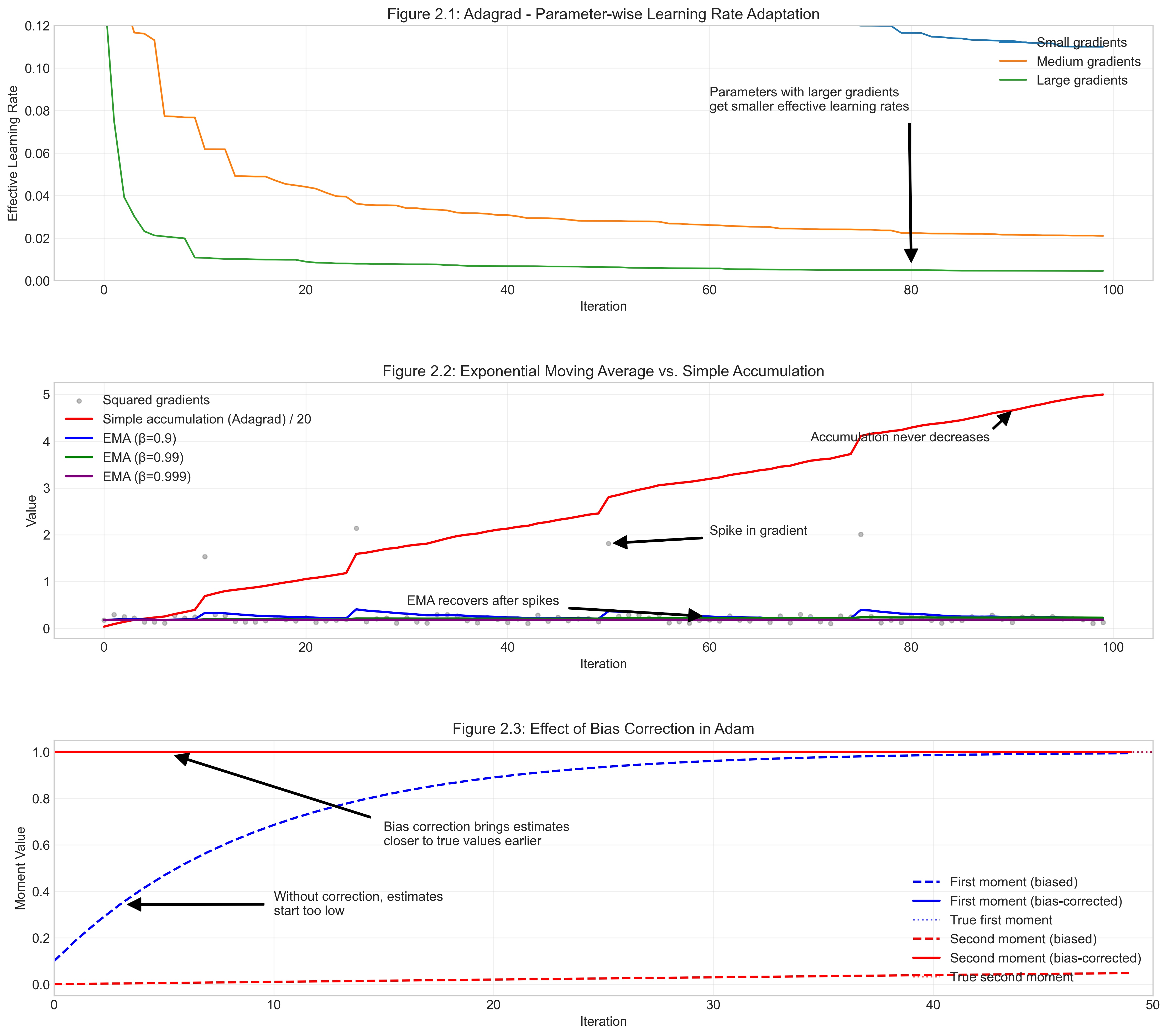
• Shows: Effective learning rate ($\alpha / \sqrt{G_{t,ii}+\epsilon}$) for two parameters.
• Takeaway:
  • Parameter with larger gradients (green) sees LR decay faster.
  • Parameter with smaller gradients (blue) maintains higher LR longer.
  • Illustrates parameter-specific adaptation.
  • Hints at the potential for LR to vanish for all parameters eventually.

Slide 10: Figure - Accumulation vs EMA

• Shows: Denominator term behavior.
  • Adagrad (red): Sum of squares ($G_{t,ii}$) grows monotonically.
  • Adam (blue, green, purple): EMA of squares ($v_t$, uncorrected) stabilizes, forgets old gradients. Different $\beta_2$ values control smoothing/memory.
• Takeaway: Adam’s EMA approach prevents the learning rate from vanishing permanently, unlike Adagrad’s accumulation.

Slide 11: Figure - Adam Bias Correction

• Shows: Impact of bias correction on moment estimates ($m_t, v_t$).
  • Dashed lines: Uncorrected estimates ($m_t, v_t$) start near zero and slowly ramp up.
  • Solid lines: Bias-corrected estimates ($\hat{m}_t, \hat{v}_t$) converge to true values much faster.
• Takeaway: Bias correction is crucial early in training for Adam to use meaningful moment estimates and avoid overly small effective learning rates initially.

Slide 12: Theory - Assumptions

• Goal: Analyze convergence $\mathbb{E}[|\nabla L(w)|^2] \to 0$.
• Setup: $L(w) = \mathbb{E}_{z \sim \mathcal{D}}[\ell(w, z)]$
• Assumption 1: Lower Bounded: $L(w) \geq L_* $ for some finite $L_* $. (Prevents divergence to $-\infty$).
• Assumption 2: Bounded Gradients ($\ell_\infty$ norm): $|\nabla \ell(w, z)|_\infty \leq R$ for all $w, z$.
  • $\|x\|_\infty = \max_i |x_i|$.
  • Needed because methods adapt coordinate-wise. Bounds per-coordinate gradient magnitude. (Contrast with typical SGD analysis using $\ell_2$ bounds on variance).
• Assumption 3: Smoothness: $L(w)$ is $L$-smooth (Lipschitz gradient).
  • $|\nabla L(w) - \nabla L(w’)|_2 \leq L|w - w’|_2$. Ensures gradient doesn’t change too rapidly.

Slide 13: Theory - Convergence Measure

• Problem Type: Generally non-convex (e.g., deep learning).
• Goal: Find a stationary point where $\nabla L(w) \approx 0$.
• Measure: Expected squared norm of the gradient: $\mathbb{E}[|\nabla L(w)|^2]$.
• Stochasticity: Iterates $w_t$ are random variables. Analyze a randomly chosen iterate $w_{\tau_N}$ from $t=0, …, N-1$.
  • Sampling distribution $P[\tau_N=j]$ might be uniform or weighted (e.g., for Adam w/ momentum, weights recent steps less: $P[\tau_N = j] \propto (1 - \beta_1^{N-j})$).
• Typical Bound Form: $\mathbb{E}[|\nabla L(w_{\tau_N})|^2] \leq \text{Term}_1(\text{Init Error}) + \text{Term}_2(\text{Noise/Variance})$.
  • Compare to SGD: Init Error $\sim O(1/N)$, Noise $\sim O(\sigma^2/N)$. We expect $O(1/\sqrt{N})$ or similar for adaptive methods with constant LR.

Slide 14: Theory - Adagrad Result (Défossez et al. 2022)

• Bound (Constant $\alpha$): \(\mathbb{E}[\|\nabla L(w_{\tau_N})\|^2] \leq \underbrace{\frac{2R(L(w_0) - L_*)}{\alpha\sqrt{N}}}_{\text{Init Term}} + \underbrace{\frac{1}{\sqrt{N}}\left(4dR^2 + \alpha dRL\right)\ln\left(1 + \frac{NR^2}{\epsilon}\right)}_{\text{Noise Term}}\)
• Rate: $O(d \ln(N) / \sqrt{N})$.
• Interpretation:
  • Initialization term decays as $O(1/\sqrt{N})$.
  • Noise term decays as $O(d \ln(N) / \sqrt{N})$.
  • Dimension Dependence: Bound includes $d$. Potentially worse than SGD if gradient variance $\sigma^2$ doesn’t scale linearly with $d$. (If $|g|_2^2 \approx d R^2$, then dependence is similar to SGD variance term).
  • $\alpha$ trade-off: Larger $\alpha$ -> faster init decay, larger noise term.
  • No need to decay $\alpha$ for convergence (adaptation handles it), unlike SGD.

Slide 15: Theory - Adam Result (Défossez et al. 2022) - Setup

• Requires Modification for Analysis: Uses simplified step size $\alpha_t = \alpha(1-\beta_1) \sqrt{\frac{1-\beta_2^t}{1-\beta_2}}$.
  • Removes bias correction for $m_t$, keeps for $v_t$. Claimed minimal practical impact.
• Focus: Result for Adam without momentum ($\beta_1 = 0$).
  • $\alpha_t$ simplifies to $\alpha \sqrt{\frac{1-\beta_2^t}{1-\beta_2}}$.

Slide 16: Theory - Adam Result ($\beta_1=0$)

• Bound: \(\mathbb{E}[\|\nabla L(w_{\tau_N})\|^2] \leq \underbrace{\frac{2R(L(w_0) - L_*)}{\alpha N}}_{\text{Init Term}} + \underbrace{E \cdot \frac{1}{N}\ln\left(1 + \frac{R^2}{(1-\beta_2)\epsilon}\right)}_{\text{Noise Term (Decaying)}} - \underbrace{E \cdot \ln(\beta_2)}_{\text{Noise Term (Constant)}}\) where $E = \frac{4dR^2}{\sqrt{1-\beta_2}} + \frac{\alpha dRL}{1-\beta_2}$.
• Interpretation:
  • Faster Init Decay: $O(1/N)$ vs Adagrad’s $O(1/\sqrt{N})$.
  • Noise Floor: Presence of constant term $-E \ln(\beta_2)$ means bound does not go to zero as $N \to \infty$ with fixed hyperparameters. Convergence is to a non-zero error level.
  • Role of $\beta_2$: Complicated trade-off in $E$ and $\ln(\beta_2)$.
  • Role of $\alpha$: Similar trade-off as Adagrad, appears in $E$.
• Adam vs Adagrad “Twins”:
  • Adam (fixed params) ~ Constant LR SGD (fast initial, non-convergent).
  • Adagrad ~ Decaying LR SGD (slower initial, convergent).
  • Adam can match Adagrad’s $O(d \ln(N) / \sqrt{N})$ rate if $\alpha \sim 1/\sqrt{N}$ and $\beta_2 = 1 - 1/N$ (i.e., scheduling).

Slide 17: Theory - Impact of Momentum ($\beta_1 > 0$)

• Bound (Complex): \(\mathbb{E}[\|\nabla L(w_{\tau_N})\|^2] \leq \frac{2R(L(w_0) - L_*)}{\alpha\tilde{N}} + E_{\beta_1}\left(\dots\right)\)
  • $\tilde{N} = N - \frac{\beta_1}{1-\beta_1} < N$ (Effective iterations reduced).
  • $E_{\beta_1}$ term is larger and more complex than $E$ for $\beta_1=0$. Contains terms like $(1-\beta_1)^{-1}$, $(1-\beta_1/\beta_2)^{-1}$, etc.
• Interpretation:
  • Theory vs Practice Gap: Theoretical bounds worsen with momentum ($\beta_1 > 0$). Effective iterations decrease, constant factors increase.
  • Improvement (Défossez et al.): Show dependence on momentum is $O((1-\beta_1)^{-1})$, much better than previous theory ($O((1-\beta_1)^{-3 \text{ to } -5})$). Momentum is less detrimental theoretically than previously thought.
  • Still implies $\beta_1 = 0$ gives best worst-case guarantee.

Slide 18: Implementation - Manual Adagrad

def adagrad_update(params, grads, state, lr=0.01, eps=1e-8):
    for i, (param, grad) in enumerate(zip(params, grads)):
        if len(state) <= i: state.append(torch.zeros_like(param))
        # Accumulate squared gradients
        state[i].add_(grad * grad) # G_t += g_t^2
        # Compute update
        std = torch.sqrt(state[i] + eps) # sqrt(G_t + eps)
        param.addcdiv_(grad, std, value=-lr) # w_t = w_{t-1} - lr * g_t / std
    return params, state

• Maintains state list for $G_{t,ii}$ accumulators.

Slide 19: Implementation - Manual Adam

def adam_update(params, grads, m_state, v_state, lr=0.001,
                beta1=0.9, beta2=0.999, eps=1e-8, t=1):
    bias_correction1 = 1 - beta1**t
    bias_correction2 = 1 - beta2**t
    for i, (param, grad) in enumerate(zip(params, grads)):
        if len(m_state) <= i:
            m_state.append(torch.zeros_like(param))
            v_state.append(torch.zeros_like(param))
        # Update biased moments
        m_state[i].mul_(beta1).add_(grad, alpha=1-beta1) # m_t = b1*m_{t-1} + (1-b1)*g_t
        v_state[i].mul_(beta2).add_(grad * grad, alpha=1-beta2) # v_t = b2*v_{t-1} + (1-b2)*g_t^2
        # Bias correction
        m_hat = m_state[i] / bias_correction1
        v_hat = v_state[i] / bias_correction2
        # Update parameters
        param.addcdiv_(m_hat, torch.sqrt(v_hat) + eps, value=-lr) # w_t = w_{t-1} - lr * m_hat / (sqrt(v_hat)+eps)
    return params, m_state, v_state

• Maintains m_state and v_state lists. Needs iteration count t.

Slide 20: Implementation - Manual AdamW

def adamw_update(params, grads, m_state, v_state, lr=0.001,
                 beta1=0.9, beta2=0.999, eps=1e-8, weight_decay=0.01, t=1):
    bias_correction1 = 1 - beta1**t
    bias_correction2 = 1 - beta2**t
    for i, (param, grad) in enumerate(zip(params, grads)):
        if len(m_state) <= i:
            m_state.append(torch.zeros_like(param))
            v_state.append(torch.zeros_like(param))
        # *** Decoupled Weight Decay ***
        param.mul_(1 - lr * weight_decay) # w = w * (1 - lr*wd)
        # Update biased moments (using original gradient)
        m_state[i].mul_(beta1).add_(grad, alpha=1-beta1)
        v_state[i].mul_(beta2).add_(grad * grad, alpha=1-beta2)
        # Bias correction
        m_hat = m_state[i] / bias_correction1
        v_hat = v_state[i] / bias_correction2
        # Update parameters (Adam step)
        param.addcdiv_(m_hat, torch.sqrt(v_hat) + eps, value=-lr)
    return params, m_state, v_state

• Key difference: param.mul_(1 - lr * weight_decay) applied before the Adam update.

Slide 21: Implementation - PyTorch Usage

import torch.optim as optim

# Assume model, dataloader, criterion exist

# Adagrad
optimizer = optim.Adagrad(model.parameters(), lr=0.01)

# Adam
optimizer = optim.Adam(model.parameters(), lr=0.001, betas=(0.9, 0.999), eps=1e-8)

# AdamW
optimizer = optim.AdamW(model.parameters(), lr=0.001, betas=(0.9, 0.999),
                        eps=1e-8, weight_decay=0.01)

# Standard Training Loop Snippet
for inputs, labels in dataloader:
    optimizer.zero_grad()    # Clear previous gradients
    outputs = model(inputs)  # Forward pass
    loss = criterion(outputs, labels) # Compute loss
    loss.backward()          # Backward pass (compute gradients)
    optimizer.step()         # Update parameters

• Use built-in torch.optim classes. Standard zero_grad(), backward(), step() pattern.

Slide 22: MWE - Experiment Setup

• Goal: Empirically compare SGD (w/ mom), Adagrad, Adam, AdamW.
• Task: Fashion MNIST classification (10 classes, grayscale images).
• Model: Simple 3-layer Feedforward Neural Network (Flatten -> Linear(784, 256) -> ReLU -> Linear(256, 128) -> ReLU -> Linear(128, 10)).
• Optimizers Compared:
  • SGD: lr=0.01, momentum=0.9, weight_decay=1e-4
  • Adagrad: lr=0.01
  • Adam: lr=0.001, betas=(0.9, 0.999), eps=1e-8
  • AdamW: lr=0.001, betas=(0.9, 0.999), weight_decay=1e-4, eps=1e-8
• Metrics: Train/Validation Loss & Accuracy over 20 epochs. Time per epoch.

Slide 23: MWE - Results: Timing

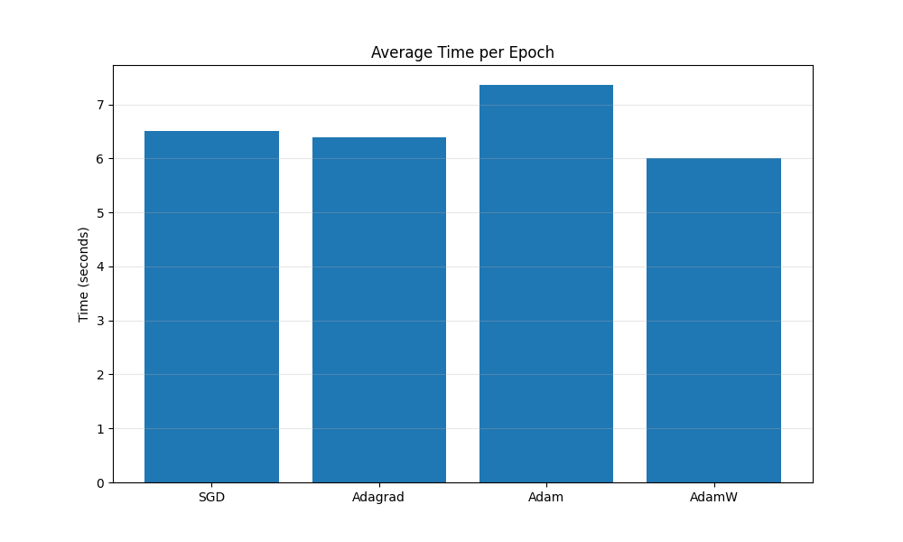
• Observation: All optimizers have roughly similar computational cost per epoch on this simple setup. Adaptive methods might have slightly higher overhead due to maintaining and updating moment estimates, but often not significantly so. (Actual results may vary).

Slide 24: MWE - Results: Performance

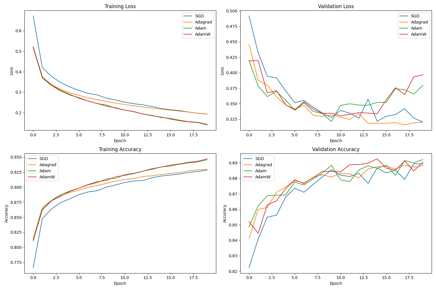
• Observation (Example):
  • Adaptive methods (Adam, AdamW, Adagrad) tend to converge faster initially in terms of loss reduction and accuracy gain compared to SGD w/ momentum (with these specific hyperparameters).
  • Adam/AdamW often perform very similarly.
  • Final performance might be comparable, or one method might slightly edge out others. AdamW might show better validation performance due to improved regularization.
• !! CRITICAL CAVEAT !!

Slide 25: MWE - IMPORTANT Caveats

• DON’T OVERGENERALIZE: Results are highly dependent on:
  • Problem/Dataset (Fashion MNIST is relatively simple).
  • Model Architecture.
  • Hyperparameter Tuning (LR, betas, weight decay are CRITICAL). We used specific defaults/common values.
• Benchmarking is HARD: Comparing optimizers fairly requires extensive tuning and multiple datasets/tasks.
  • See work like Algoperf benchmark and related papers (e.g., Choi et al., 2020, Schmidt et al., 2021 on benchmarking difficulties).
• Conclusion: These plots provide one data point. Adaptive methods are popular defaults (esp. Adam/AdamW) bc they often work well “out-of-the-box” across many tasks, but well-tuned SGD can still be competitive or better.