Basic idea behind flash attention (V1)
The naive implementation of self-attention on a GPU is slow, not because of the number of floating-point operations (FLOPs), but because of memory accesses. Flash attention is a way to reduce memory access while still computing exact attention.
Recall the attention operation is defined as:
\[S = QK^T, \quad P = \text{softmax}(S), \quad O = PV\]Here, for a sequence of length $N$ and a head dimension $d$, the query $Q$, key $K$, and value $V$ matrices are size $N \times d$. The attention matrix $S$ and the probability matrix $P$ are both size $N \times N$.
Why is the naive implementation slow? A GPU has a memory hierarchy. A small amount of very fast on-chip memory (SRAM) is available to the compute cores. A much larger, but slower, pool of memory (HBM, or High-Bandwidth Memory) is off-chip. Most operations in a deep learning model are “memory-bound,” meaning their speed is limited by the time it takes to move data between HBM and SRAM, not by the arithmetic computations performed in SRAM. I recommend reading this blog post by Horace He for a quick primer on compute, memory, and overhead in deep learning.
The standard implementation of attention materializes the $N \times N$ matrices $S$ and $P$ in HBM. This involves:
- Reading $Q$ and $K$ from HBM.
- Computing $S=QK^T$ and writing $S$ back to HBM.
- Reading $S$ from HBM.
- Computing $P=\text{softmax}(S)$ and writing $P$ back to HBM.
- Reading $P$ and $V$ from HBM.
- Computing $O=PV$ and writing $O$ back to HBM.
For long sequences ($N \gg d$), the $O(N^2)$ memory reads and writes for $S$ and $P$ dominate the runtime.
The problem is the HBM traffic. Let B be the bytes per element. The implementation writes and then reads the $N \times N$ matrix $S$ (totaling $2N^2B$ bytes), and then writes and reads the $N \times N$ matrix $P$ (another $2N^2B$ bytes). These four operations, which transfer data to and from the large but slow HBM, dominate the $O(NdB)$ traffic from reading the initial inputs $Q, K, V$ and writing the final output $O$. The total HBM access is thus $O(N^2 + Nd)$ bytes.
Flash attention (V1)
FlashAttention computes the same attention output $O$ without writing the full $N \times N$ matrices $S$ and $P$ to HBM. It achieves this by restructuring the computation using two techniques: tiling and online softmax. The idea is to perform the entire attention calculation in smaller blocks, keeping all intermediate products within the fast on-chip SRAM until the final block of the output $O$ is ready. This post, again by Horace, is useful for seeing why tiling is a good idea.
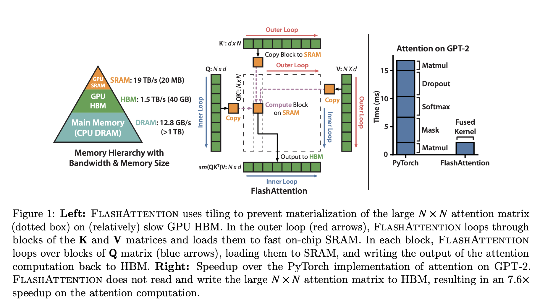 Figure 1 from the FlashAttention paper.
NOTE: this post is about the original FlashAttention paper. There are now three versions of FlashAttention, but we’ll stick with V1 for simplicity.
Tiling
The computation is broken into blocks. The matrices $Q, K, V$ are partitioned into smaller sub-matrices. The algorithm iterates through blocks of $K$ and $V$, loading them into SRAM. Within this outer loop, it iterates through blocks of $Q$.
A simplified view of the loops:
// O is the final output matrix, initialized to zero
// l, m are statistics for the online softmax, initialized
for each block K_j, V_j in K, V:
  Load K_j, V_j into fast SRAM
  for each block Q_i in Q:
    Load Q_i, O_i, l_i, m_i into fast SRAM
    // Core computation, all on-chip
    Compute S_ij = Q_i @ K_j^T
    Compute P_ij = softmax(S_ij) // (This is a simplification, see next section)
    Compute O_ij = P_ij @ V_j
    // Update the output block O_i with the new result
    Update O_i using O_ij and softmax statistics
    // Write the updated O_i, l_i, m_i back to HBM
    Write O_i, l_i, m_i to HBM
This tiled structure changes the memory access pattern. The algorithm iterates through $K$ and $V$ in blocks, reading each element from HBM only once. The critical part is the inner loop. For each block of $K_j$ loaded into SRAM, the algorithm must iterate through all blocks of $Q$ to compute the corresponding updates to the output. This means the algorithm makes multiple passes over the $Q$ matrix. The number of passes is determined by the number of blocks in $K$, which is $T = N/B$, where $B$ is the block size. Since the on-chip SRAM of size $M$ must hold a block of $K$ (size $B \times d$), the block size $B$ is limited to $O(M/d)$. This leads to $T = O(Nd/M)$ passes. Each pass reads the entirety of $Q$ (and reads/writes blocks of $O$), resulting in HBM traffic of $O(Nd \times T) = O(N^2 d^2 / M)$ bytes. This quantity is substantially smaller than the $O(N^2)$ traffic of standard attention.
Example:
To make this concrete, consider an NVIDIA A100 GPU. Each of its Streaming Multiprocessors has 192KB of SRAM. A single kernel will use a portion of this, let’s assume a working SRAM size of M_bytes = 128KB. If we use bfloat16 precision (2 bytes per number), the effective SRAM size in elements is M = 128 * 1024 / 2 = 65,536 elements. For a typical head dimension d=64, $d^2 = 4096$. The reduction factor in memory accesses is approximately $M/d^2 = 65536 / 4096 = 16$. FlashAttention performs roughly 16 times fewer HBM accesses than the standard implementation. For $d=128$, the factor is $M/d^2 = 65536 / 16384 = 4$.
Online Softmax
The softmax function is applied row-wise. For a row $x_i$ of the attention score matrix $S$, the output is $\text{softmax}(x_i)_j = \frac{e^{x_{ij}}}{\sum_k e^{x_{ik}}}$. The denominator requires a sum over the entire row, which seems to prevent block-wise computation.
The “online softmax” algorithm solves this. It computes the exact softmax by maintaining two running statistics for each row $i$: the maximum value seen so far ($m_i$) and the sum of the exponentials of the scaled values ($l_i$). For numerical stability, softmax is computed as:
\[m(x) = \max_j(x_j), \quad l(x) = \sum_j e^{x_j - m(x)}, \quad \text{softmax}(x)_j = \frac{e^{x_j - m(x)}}{l(x)}\]When processing the $j$-th block of a row $x_i$, which we denote $x_{i,j}$, we can update the statistics and the output $O_i$ as follows:
- Compute the local statistics for the current block: $m_{i,j} = \max_k(x_{ik})$ and $l_{i,j} = \sum_k e^{x_{ik} - m_{i,j}}$.
- Compute the new global maximum: $m_i^{\text{new}} = \max(m_i^{\text{old}}, m_{i,j})$.
-
Update the output value using the old and new statistics:
\[O_i^{\text{new}} = \frac{1}{l_i^{\text{new}}} \left( l_i^{\text{old}} e^{m_i^{\text{old}} - m_i^{\text{new}}} O_i^{\text{old}} + l_{i,j} e^{m_{i,j} - m_i^{\text{new}}} O_{i,j} \right)\]where $O_{i,j}$ is the attention output computed using only the current block of $K$ and $V$, and $l_i^{\text{new}}$ is the appropriately rescaled sum.
It’s straightforward to see that by storing and updating these two scalars ($m_i, l_i$) per row, Flash attention can produce the exact output of the softmax operator without needing the whole row at once.
The Backward Pass and Recomputation
The backward pass of attention requires the gradients $\frac{\partial L}{\partial Q}, \frac{\partial L}{\partial K}, \frac{\partial L}{\partial V}$. Computing these requires the matrix $P$ from the forward pass. A standard implementation would read the saved $N \times N$ matrix $P$ from HBM, incurring the same memory bottleneck.
Flash attention avoids this by not storing $P$ at all. Instead, during the backward pass, it recomputes the necessary blocks of the attention matrix $P$ as needed. It does this by loading the required blocks of $Q$, $K$, and $V$ from HBM back into SRAM. The only values saved from the forward pass are the final output $O$ $(N \times d)$ and the online softmax statistics ($m, l$).
This introduces more FLOPs, as parts of the forward pass are re-done. However, since the operation is memory-bound, the time spent on these extra FLOPs is insignificant compared to the time saved by avoiding a massive read from HBM.