Getting the hang of policy gradients by reframing optimization as RL
We can gain insight into Reinforcement Learning (RL) training mechanisms by taking a general optimization problem and reframing it as a “stateless RL problem.” In this reframing, the task is to find optimal parameters for a probability distribution that generates candidate solutions. The distribution’s parameters are adjusted based on rewards received for sampled solutions, aiming to increase the probability of generating high-reward solutions. This perspective isolates aspects of policy optimization from complexities such as state-dependent decision making.
Note: while writing this I remembered that Mr. Ben Recht wrote a blog post that considered a similar reframing back in 2018.
From Optimization to a Stateless RL
Consider the general problem of finding a vector $w$ that minimizes a loss function $L(w)$:
\[\min_w L(w)\]$L(w)$ can be a deterministic function of $w$. Alternatively, $L(w)$ might represent an expected loss,
\[L(w) = E_{z \sim D_z}[\ell(w,z)]\]where $\ell(w,z)$ is a loss computed for a specific data sample $z$ drawn from a distribution $D_z$.
To transform this into an RL problem, we shift from directly seeking an optimal $w$ to optimizing the parameters $\theta$ of a policy $\pi_\theta(w)$. The policy $\pi_\theta(w)$ is a probability distribution that generates candidate solutions $w$. The RL objective is then to find parameters $\theta$ that maximize the expected reward $J(\theta)$ obtained from these solutions:
\[J(\theta) = E_{w \sim \pi_\theta(w)}[R(w)]\]If the policy is $\pi_\theta(w) = N(w|\mu, \sigma^2)$ and the reward is $R(w) = -L(w)$, with $L(w)$ uniquely minimized at $w^* $, then $J(\theta)$ is maximized as the policy mean $\mu$ approaches $w^*$ and the standard deviation $\sigma$ approaches $0^+$. In this limit, the policy effectively concentrates its mass at $w^* $.
In this construction:
- The policy $\pi_\theta(w)$, parameterized by $\theta$, is the distribution used to sample candidate solutions $w$.
- An action corresponds to sampling a solution $w$ from $\pi_\theta(w)$.
- The environment is effectively stateless because the reward $R(w)$ for a sampled solution $w$ depends only on $w$.
The definition of the reward $R(w)$ is derived from the original optimization problem. If the goal is to minimize $L(w)$, one reward definition is $R(w) = -L(w)$. If the loss is stochastic, $\ell(w,z)$, then the reward can also be stochastic, for example, $R(w,z) = -\ell(w,z)$. In this stochastic reward case, the objective becomes $J(\theta) = E_{w \sim \pi_\theta(w)}[E_{z \sim D_z}[R(w,z)]]$.
Example Reward Formulations
The way $R(w)$ (or $R(w,z)$) is defined based on $L(w)$ or $\ell(w,z)$ directly influences the information available to the learning algorithm. To explore these effects, we consider several reward structures:
- True Reward: $R(w) = -L(w)$.
- This reward provides direct information about $L(w)$ for each sampled $w$.
- Unbiased Randomized Reward: $R(w,z) = -\ell(w,z)$, where $z \sim D_z$.
- This reward uses individual data instances $z$. $R(w,z)$ is noisy, but $\mathbb{E}_z[R(w,z)] = -L(w)$.
- Proxy Rewards (via a fixed batch): $R(w) = -\frac{1}{|S_{train}|} \sum_{z_i \in S_{train}} \ell(w,z_i)$. $S_{train}$ is a fixed data batch.
- If $S_{train}$ is unrepresentative, optimizing this $R(w)$ illustrates RL with a learned proxy reward.
- Sparse Rewards: $R(w) = \mathbb{1}_{-L(w) > \text{tol}}$, where $\text{tol}$ is a threshold.
- This yields a binary signal. If the condition is met infrequently, the reward is sparse.
The Policy Gradient in a Stateless Setting
The Policy Gradient Theorem (PGT) provides a method for computing $\nabla_\theta J(\theta)$. (A PGT derivation is in a previous post). For the stateless problem, the policy gradient is:
\[\nabla_\theta J(\theta) = \mathbb{E}_{w \sim \pi_\theta(w), z \sim D_z}[ \nabla_\theta \log \pi_\theta(w) R(w,z) ] \quad (*)\](If $R(w)$ is deterministic, omit expectation over $z$). A stochastic estimate of $\nabla_\theta J(\theta)$ is $\hat{g}_t = \nabla_\theta \log \pi_\theta(w_t) R(w_t, z_t)$, using samples $w_t \sim \pi_{\theta_t}(w)$ and $z_t \sim D_z$. Policy parameters can then be updated via stochastic gradient ascent:
\[\theta \leftarrow \theta + \alpha \hat{g}_t\]Properties of the Policy Gradient Estimator
The estimator $\hat{g}_t = \nabla_\theta \log \pi_\theta(w_t) R(w_t, z_t)$ is an unbiased estimate of $\nabla_\theta J(\theta)$. The variance of this estimator, $\text{Var}(\hat{g}_t) = \mathbb{E}[(\nabla_\theta \log \pi_\theta(w) R(w,z))^2] - (\nabla_\theta J(\theta))^2$, can be large. This variance impacts learning stability and speed.
For example, consider a policy $\pi_\theta(w) = N(w | \mu, \sigma^2 I_d)$ for $w \in \mathbb{R}^d$. Let parameters be $\theta = (\mu, \psi)$, where $\psi = \log\sigma$ ensures $\sigma = e^\psi > 0$. The score function for $\mu$ is
\[\nabla_\mu \log \pi_\theta(w) = (w-\mu)/\sigma^2.\]The variance of the $\mu$-component of $\hat{g}_t$, $\hat{g}_{\mu,t}$, involves $E[|(w-\mu)/\sigma^2|^2 R(w,z)^2]$. The term $E[|w-\mu|^2/\sigma^4]$ contributes a factor scaling as $d/\sigma^2$. Thus, $\text{Var}(\hat{g}_{\mu,t})$ can scale proportionally to $d/\sigma^2$ multiplied by terms related to $R(w,z)$. This $1/\sigma^2$ dependence shows that as $\sigma \to 0$ (exploitation), $\text{Var}(\hat{g}_{\mu,t})$ can increase if $R(w,z)$ does not also diminish appropriately as $w \to \mu$.
The score for $\psi=\log\sigma$ is
\[\nabla_{\psi} \log \pi_\theta(w) = (\|w-\mu\|^2/\sigma^2 - d),\]where $d$ is the dimension of $w$. The variance of its gradient estimate also depends on $R(w,z)$ and $\sigma$.
Note that an interesting consequence of optimization $L$ via the PGT approach is that $R(w,z)$ can be non-differentiable with respect to $w$. Indeed, we only need to calculate the gradient for policy parameters. This flexibility is exchanged for managing the variance of $\hat{g}_t$. Well, that and the fact that $J$ is generally nonconvex in $\sigma$, even if $L$ is convex.
Aside: Connection to Gaussian Smoothing
If the policy is $w \sim N(\mu, \sigma_0^2 I_d)$ with fixed $\sigma_0^2$ (so $\theta = \mu$), and $R(w) = -L(w)$, then
\[J(\mu) = E_{w \sim N(\mu, \sigma_0^2 I_d)}[-L(w)] = -L_{\sigma_0}(\mu),\]where
\[L_{\sigma_0}(\mu) = E_{w \sim N(\mu, \sigma_0^2 I_d)}[L(w)]\]is the Gaussian-smoothing of the function $L(\cdot)$ evaluated at $\mu$. The policy gradient $\nabla_\mu J(\mu)$ is then $-\nabla_\mu L_{\sigma_0}(\mu)$. Thus, PGT here performs stochastic gradient descent on a smoothed version of $L$. This links PGT to zeroth-order optimization methods.
Variance of the gradient, stepsize selection, and gradient clipping
Recall that we wish to maximize $J(\theta)$ via the stochastic gradient ascent update $\theta \leftarrow \theta + \alpha \hat{g}_t$. Two primary considerations for SGA are the variance of $\hat{g}_t$ and the selection of stepsize $\alpha$.
Variance Reduction
Baselines: In the stateless setting,
\[V^{\pi_\theta} = E_{w \sim \pi_\theta(w)}[R(w)]\]is the expected reward under the policy. The advantage is
\[A^{\pi_\theta}(w') = R(w') - V^{\pi_\theta}.\]Subtracting a baseline $b_t \approx V^{\pi_\theta}$ from the reward:
\[\hat{g}_t = \nabla_\theta \log \pi_\theta(w_t) (R(w_t, z_t) - b_t)\]One way to estimate $V^{\pi_\theta}$ online is using an exponential moving average of rewards. This provides $b_t$. The centered term $(R(w_t,z_t) - b_t)$ can yield a lower variance $\hat{g}_t$.
Batch Gradient Estimator: One can average $\hat{g}_t$ over a mini-batch of $N_s$ independent samples $w_j \sim \pi_\theta(w)$ (each with its own $R(w_j)$ or $R(w_j, z_j)$). This forms $\bar{g}_t = \frac{1}{N_s} \sum_{j=1}^{N_s} \hat{g}_{t,j}$. In this case,
\[\text{Var}(\bar{g}_t) = \text{Var}(\text{single sample } \hat{g}_t)/N_s.\]This reduces variance at the cost of $N_s$ reward evaluations per policy update.
Stepsize Selection and Convergence
The objective $J(\theta)$ is generally non-convex. For non-convex $J(\theta)$, convergence rate analysis focuses on metrics like $E[|\nabla J(\theta_k)|^2] \to 0$ (or to a noise floor for constant $\alpha$). In more restricted settings, for example, if $J(\theta)$ is (locally) strongly convex around an optimum $\theta^*$, metrics like $E[|\theta_k-\theta^*|^2]$ or $J(\theta^*) - J(\theta_k)$ can be analyzed. The stepsize (or learning rate1) $\alpha$ affects convergence. (if none of this is familiar to you, see my lecture notes on stochastic gradient descent for mean estimation)
-
Constant Stepsize: For a constant $\alpha$, $\theta_k$ oscillates around a region where $\nabla J(\theta) \approx 0$. A convergence metric $M_k(\alpha)$ (e.g., $E[|\nabla J(\theta_k)|^2]$ for non-convex or $E[|\theta_k-\theta^*|^2]$ for locally convex) usually scales as:
\[M_k(\alpha) \approx \frac{C_0 \cdot (\text{Initial Error})}{h(k) \cdot \alpha} + \frac{C_1 \cdot \alpha \cdot \text{Var}(\text{single sample } \hat{g}_t)}{N_s}\]where $h$ is some function of $k$ (e.g., $k^{-1/2}$) and $N_s$ is the batch size for $\hat{g}_t$ ($N_s=1$ if no batching). As $k \to \infty$, the first term (bias reduction) vanishes, leaving the second term (noise floor). A larger $\alpha$ speeds initial progress but gives a higher noise floor.
-
Diminishing Stepsize: For $M_k(\alpha_k) \to 0$, $\alpha_k$ must diminish, for instance, satisfying the Robbins-Monro conditions: $\sum_{k=0}^\infty \alpha_k = \infty$ and $\sum_{k=0}^\infty \alpha_k^2 < \infty$.
There are of course issues with these bounds when we take $\sigma$ to zero, since the variance explodes. To actually achieve convergence, we would need to increase the batch size sufficiently fast. Or, we could
Clip the gradients
Gradient clipping replaces $\hat{g}_t$ with $c\frac{\hat{g}_t}{||\hat{g}_t||}$ if $||\hat{g}_t|| > c$ for a user specified constant $c$. Since the gradient of the score function explodes as $\sigma$ tends to zero, this becomes necessary.
Illustrative experiments: Policy Gradient for a Quadratic Loss
We apply these concepts to an agent (everything’s an agent now!) learning to sample $w$ to minimize
\[L(w) = \frac{1}{2}(w - w^\ast)^2\]for a target $w^\ast$.
A stochastic version of the loss is
\[\ell(w,z) = \frac{1}{2}(w -(w^\ast + z))^2,\]where $z \sim N(0, \sigma_z^2)$.
The agent’s policy $\pi_\theta(w)$ is $N(w|\mu, \sigma^2)$, for scalar $w$ (i.e., $d=1$). The learnable parameters are $\theta = (\mu, \psi)$, where $\psi = \log\sigma$. This parameterization ensures $\sigma = e^\psi > 0$ when $\psi$ is optimized without constraints.
We now present results from numerical experiments applying the policy gradient approach to the quadratic loss $L(w) = \frac{1}{2}(w - w^\ast)^2$ with target $w^\ast=5.0$. All experiments start from an initial policy $N(0,4)$ and use gradient clipping with norm 10.0. We examine the five reward formulations (R1-R4). For R1 and R2, we investigate the effects of learning rate, baselines, diminishing stepsizes, and batching. For R3, R4, and R5, we show specific illustrative runs.
R1: True Reward
The reward is $R(w) = -L(w) = -\frac{1}{2}(w - w^\ast)^2$. Runs use $10^4$ episodes.
Learning Rate Comparison (Set A):
 Figure 1: R1 (True Reward) - Learning Rate Comparison. Compares constant $\alpha \in {0.01, 0.001, 0.0001}$. All use EMA baseline, $N_s=1$. Higher $\alpha$ converges $\mu$ faster towards $w^\ast=5.0$ and decreases $\sigma$ faster. Lower $\alpha$ converges slower.
Baseline Comparison (Set B):
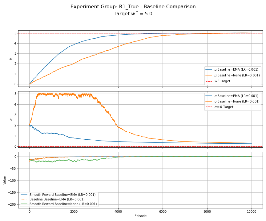 Figure 2: R1 (True Reward) - Baseline Comparison. Compares EMA baseline vs. no baseline ($b_t=0$) for $\alpha=0.001$, $N_s=1$. The EMA baseline stabilizes the decrease of $\sigma$, avoiding the large initial increase seen without a baseline.
Stepsize Schedule Comparison (Set C):
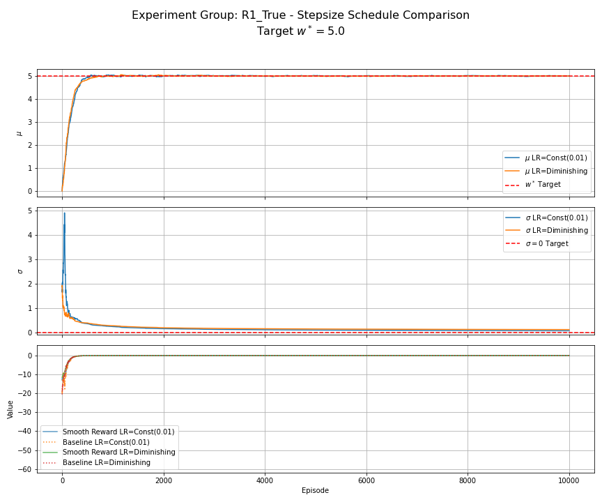 Figure 3: R1 (True Reward) - Stepsize Schedule Comparison. Compares constant $\alpha=0.01$ vs. a diminishing schedule starting at $\alpha_0=0.01$. Both use EMA baseline, $N_s=1$. Performance is comparable over this number of episodes; the diminishing schedule shows slightly less oscillation in $\mu$ near the end.
Batch Gradient Estimator Comparison (Set D):
 Figure 4: R1 (True Reward) - Batch Gradient Comparison. Compares $N_s=1$ vs. $N_s=10$. Both use $\alpha=0.001$, EMA baseline. Using $N_s=10$ results in visibly smoother trajectories for $\mu$ and $\sigma$, demonstrating variance reduction per update.
R2: Randomized Reward
The reward is $R(w,z) = -\ell(w,z) = -(\frac{1}{2}(w - (w^\ast+z))^2)$, where $z \sim N(0, 1)$. Runs use $10^4$ episodes.
Learning Rate Comparison (Set A):
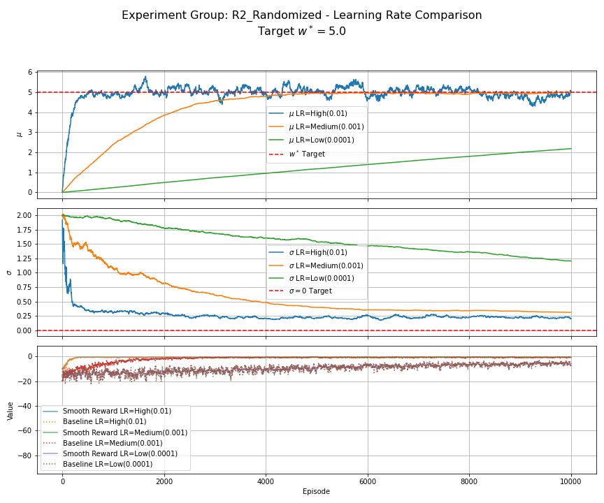 Figure 5: R2 (Randomized Reward) - Learning Rate Comparison. Compares constant $\alpha \in {0.01, 0.001, 0.0001}$. All use EMA baseline, $N_s=1$. Higher $\alpha$ converges faster but exhibits significant oscillations around $w^\ast=5.0$ (noise floor). Lower $\alpha$ reduces oscillation variance but converges slower.
Baseline Comparison (Set B):
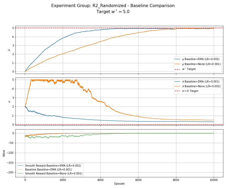 Figure 6: R2 (Randomized Reward) - Baseline Comparison. Compares EMA baseline vs. no baseline ($b_t=0$) for $\alpha=0.001$, $N_s=1$. The EMA baseline enables stable convergence of $\mu$ and $\sigma$. Without the baseline, learning is highly unstable, especially for $\sigma$.
Stepsize Schedule Comparison (Set C):
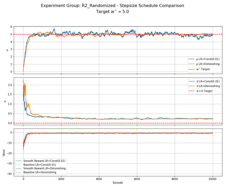 Figure 7: R2 (Randomized Reward) - Stepsize Schedule Comparison. Compares constant $\alpha=0.01$ vs. diminishing schedule starting at $\alpha_0=0.01$. Both use EMA baseline, $N_s=1$. The diminishing stepsize significantly reduces the oscillations (noise floor) seen with the constant stepsize.
Batch Gradient Estimator Comparison (Set D):
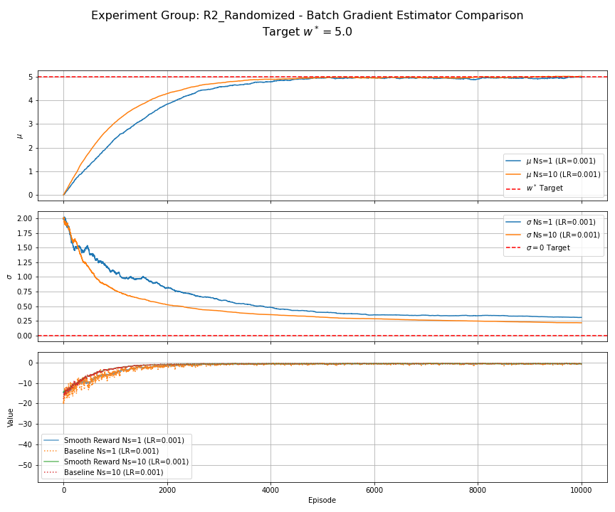 Figure 8: R2 (Randomized Reward) - Batch Gradient Comparison. Compares $N_s=1$ vs. $N_s=10$. Both use $\alpha=0.001$, EMA baseline. Using $N_s=10$ yields noticeably smoother trajectories for $\mu$ and $\sigma$, reducing the impact of reward noise.
R3: Proxy Reward Optimization (Fixed Batch)
This experiment investigates optimizing a proxy reward based on a fixed batch $S_{train}$. The reward is $R(w) = -\text{avg}_{z_i \in S_{train}}[\ell(w, z_i)]$, where $\ell(w, z_i) = \frac{1}{2}(w - (w^\ast + z_i))^2$ and $S_{train}$ contains $N_s$ samples of $z_i \sim N(0,1)$ generated once. We compare results for batch sizes $N_s=1, 5, 10, 20$. All runs use $\alpha=0.01$, EMA baseline, and $10^4$ episodes.
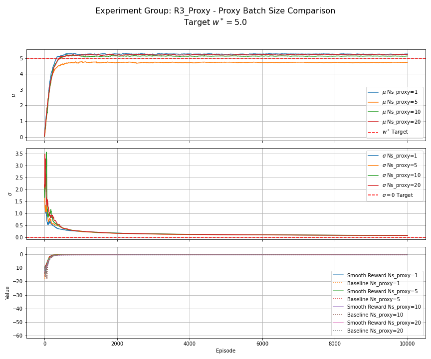 Figure 9: R3 Proxy Reward (Fixed Batch) - Batch Size Comparison. Compares optimizing the empirical average reward over fixed batches $S_{train}$ of size $N_s \in {1, 5, 10, 20}$. All use $\alpha=0.01$, EMA baseline. Convergence of $\mu$ appears closer to the true $w^\ast=5.0$ as $N_s$ increases, illustrating how optimizing a small fixed batch (a proxy objective) can lead to solutions biased away from the true optimum.
R4: Discrete Sparse Reward
The reward is $R(w) = 1$ if $(w-w^\ast)^2 < 0.25$, else $0$. We show a single run with $\alpha=0.01$, EMA baseline, $N_s=1$, for $5 \times 10^4$ episodes.
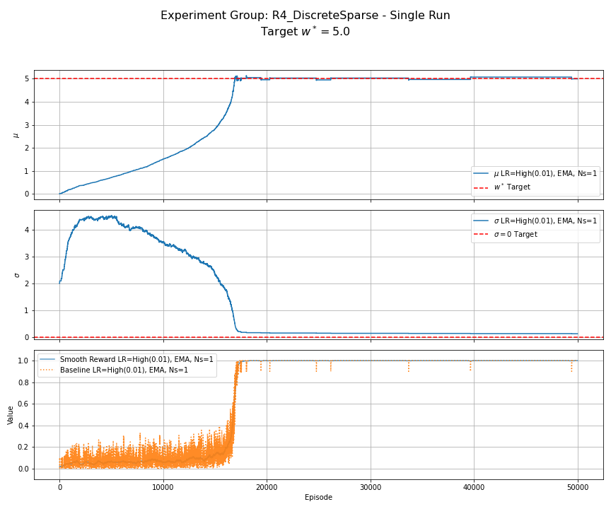 Figure 10: R4 (Discrete Sparse Reward) - Single Run. Reward is 1 if $|w-w^\ast|<0.5$, else 0. Uses $\alpha=0.01$, EMA baseline, $N_s=1$. Learning shows a long initial phase with slow progress in $\mu$ while $\sigma$ increases (exploration). Once the rewarding region is found, $\mu$ converges towards $w^\ast$ and $\sigma$ decreases.
Footnotes
-
I think I’ve completely given up and no longer care whether I say stepsize or learning rate. ↩