Notes — full feed
Basic facts about GPUs
I’ve been trying to get a better sense of how GPUs work. I’ve read a lot online, but the following posts were particularly helpful:
- Making Deep Learning Go Brrrr From First Principles
- What Shapes Do Matrix Multiplications Like?
- How to Optimize a CUDA Matmul Kernel for cuBLAS-like Performance: a Worklog
This post collects various facts I learned from these resources.
Acknowledgements: Thanks to Alex McKinney for comments on independent thread scheduling.
Table of Contents
- Compute and memory hierarchy
- Two Performance Regimes: Memory-Bound and Compute-Bound
- The Third Regime: Overhead
- Two basic strategies for increasing performance: Fusion and Tiling
- Additional Performance Considerations
Compute and memory hierarchy
A GPU’s design creates an imbalance since it can compute much faster than it can access its main memory. An NVIDIA A100 GPU, for example, can perform 19.5 trillion 32-bit floating-point operations per second (TFLOPS), but its memory bandwidth is only about 1.5 terabytes per second (TB/s). In the time it takes to read a single 4-byte number, the GPU could have performed over 50 calculations.
Below is a diagram of the compute and memory hierarchy for an NVIDIA A100 GPU. The numbers I quote for flops/s and TB/s are exclusive to A100s.
+---------------------------------------------------------------------------------+
|                               Global Memory (VRAM)                              |
|                            (~40 GB, ~1.5 TB/s on A100)                          |
+----------------------------------------+----------------------------------------+
                                         | (Slow off-chip bus)
+----------------------------------------v----------------------------------------+
|                            Streaming Multiprocessor (SM)                        |
|                     (1 of 108 SMs on an A100, each ~(19.5/108) TFLOPS)          |
|                           (2048 threads, 64 warps, 32 blocks)                   |
| +-----------------------------------------------------------------------------+ |
| |                        Shared Memory (SRAM) / L1 Cache                        |
| |                    (~192 KB on-chip workbench, 19.5 TB/s)                     |
| +-----------------------------------------------------------------------------+ |
| |                        Register File (~256 KB, ? TB/s)                        |
| +-----------------------------------------------------------------------------+ |
| |                                                                             | |
| |                //-- A "Block" of threads runs on one SM --//                | |
| | +--------------------------+ +------------------------+                     | |
| | |      Warp 0 (32 thr)     | |      Warp 1 (32 thr)   | ... (up to 32 warps)| |
| | | +----------------------+ | +----------------------+ |                     | |
| | | | Thread 0 Registers   | | | Thread 32 Registers  | |                     | |
| | | | [reg0: float]        | | | [reg0: float]        | |                     | |
| | | | [reg1: float] ...    | | | [reg1: float] ...    | |                     | |
| | | +----------------------+ | +----------------------+ |                     | |
| | +--------------------------+ +------------------------+                     | |
| |                                                                             | |
+---------------------------------------------------------------------------------+
This diagram shows the performance hierarchy.1 Global Memory (VRAM) is the large, slow, off-chip memory pool where all data initially lives. A Streaming Multiprocessor (SM) is the GPU’s unit of computation. To work, it must fetch data over the slow bus. To mitigate this, each SM has fast, on-chip Shared Memory (SRAM) with a bandwidth of 19.5 TB/s.2 Programmers use this as a manually-managed cache.
A thread is the smallest unit of execution. Each thread has a private set of Registers to hold values for immediate computation, with access speeds over ?? TB/s.3 The hardware groups threads into Warps of 32. This post analyzes performance using the simplified model of lockstep execution, where all 32 threads in a warp execute the same instruction at the same time.4 On an A100, an SM has an upper limit of 64 warps. A programmer groups threads into a Block, a grid of threads that is guaranteed to run on a single SM. A block can be one, two, or three-dimensional. For simplicity, this post will focus on square two-dimensional blocks of BLOCK_DIM x BLOCK_DIM threads, where the total number of threads cannot exceed the hardware limit of 1024. All threads in a block share access to the same on-chip Shared Memory.
The Two Performance Regimes
We analyze the performance of a kernel, which is a function launched by the host (CPU) to be executed in parallel by many GPU threads. A kernel’s performance is limited by either its memory bandwidth or its compute throughput. These two limits define the performance regimes.
An operation is memory-bound if its runtime is dictated by the speed of transferring data from Global Memory to the SM. For an operation like element-wise addition y = x + 1, the SM performs a trivial number of FLOPs for each element it reads. The SM spends most of its time idle, waiting for data.
An operation is compute-bound if its runtime is dictated by the SM’s arithmetic speed. A large matrix multiplication is the canonical example. Once data is loaded into the SM, a massive number of computations are performed. The memory bus is idle while the SM is busy.
Arithmetic Intensity (AI) is the formal metric that determines the regime. It is the ratio of work to memory traffic.
Arithmetic Intensity = Total FLOPs / Total Bytes Accessed
For the Roofline model, Total Bytes Accessed specifically counts the data transferred between Global Memory (HBM) and the on-chip SM. This is because the model evaluates a kernel’s performance against the primary bottleneck: the slow off-chip memory bus. On-chip traffic, such as from Shared Memory to registers, is not included in this calculation.
The Roofline Model plots a kernel’s achievable performance (in FLOPs per second) against its AI. The two “roofs” are the hard physical limits of the GPU.
  ^ Performance (TFLOPS)
  |
  | Memory-Bound Region ¦ Compute-Bound Region
  |                     ¦
  |                    /¦----------------------  <-- Peak Compute (~19.5 TFLOPS)
  |                   / ¦
  |                  /  ¦
  | Peak Global     /<--¦------ Inefficient Compute Roof (e.g., using scalar ops, transcendental functions)
  | Mem BW (~1.5   /    ¦
  | TB/s)         /     ¦
  |              /      ¦
  +---------------------¦---------------------------> Arithmetic Intensity (FLOPs/Byte)
                        ^
                        ¦
                  Hardware Ridge Point (~13)
The performance of a kernel is determined as follows:
- When memory-bound, the SMs are stalled waiting for data. The runtime is the time it takes to move that data:
Runtime = Bytes_Accessed / Memory_Bandwidth. The kernel’s performance is thereforePerformance = Total_FLOPs / Runtime = AI * Memory_Bandwidth. On the log-log plot, this is the diagonal line. - When compute-bound, the SMs are fully utilized. The performance is limited by their peak arithmetic throughput:
Performance = Peak_Compute_FLOPs. This is the horizontal line.
A kernel’s actual performance is the minimum of these two values. The ridge point is the AI where the two performance ceilings intersect. For the A100, this is 19.5 TFLOPS / 1.5 TB/s ≈ 13 FLOPs/Byte. A kernel must exceed this AI to become compute-bound. A kernel with AI lower than 13 operates in the memory-bound region; a kernel with AI higher than 13 operates in the compute-bound region. The goal of optimization is to increase AI to move the kernel’s operating point to the right, pushing its performance up until it hits the compute roof.
The “Peak Compute” roof of 19.5 TFLOPS is an ideal, achievable only with highly optimized instructions like Tensor Core matrix multiplications and high enough power limits. An operation can be compute-bound but still perform far below this peak. For example, a kernel with high AI that is dominated by scalar arithmetic or complex transcendental functions (sin, exp) will be limited by the throughput of those specific, slower instructions. This creates a lower effective “roof” for that kernel, as shown in the diagram. Increasing AI is necessary, but not sufficient; the FLOPs must also be efficient.
The primary strategy to increase AI is to maximize the reuse of data once it has been loaded into the SM’s fast on-chip memory. The following is a simplified model where a thread reads data from Global Memory directly into its private registers. This analysis calculates the minimum required data transfer; actual memory traffic depends on access patterns, which we will discuss later.
Consider computing C = A@B, where all matrices are N x N and use 4-byte floats.
Strategy 1: One thread computes one element C[i,j]
- FLOPs: To compute
C[i,j], the thread performs N multiply-add operations. This is2*NFLOPs. - Bytes Accessed: The thread must read row
iof A (N floats) and columnjof B (N floats). This is a total of2*Nfloats, or8*Nbytes. - Arithmetic Intensity:
(2*N FLOPs) / (8*N Bytes) = 0.25 FLOPs/Byte.
This AI is low. The kernel will be memory-bound.
Strategy 2: One thread computes a 2x2 tile of C
To compute a 2x2 tile (C[i,j], C[i,j+1], C[i+1,j], C[i+1,j+1]), the thread must perform the computation for all four elements.
- FLOPs:
4 elements * 2*N FLOPs/element = 8*NFLOPs. - Bytes Accessed: The thread must read two rows from A (
A[i,:],A[i+1,:]) and two columns from B (B[:,j],B[:,j+1]). This is2*N + 2*N = 4*Nfloats, or16*Nbytes. - Arithmetic Intensity:
(8*N FLOPs) / (16*N Bytes) = 0.5 FLOPs/Byte.
These AI values are far below the A100’s ridge point of ~13 FLOPs/Byte. This simple register-only model is insufficient to make matrix multiplication compute-bound.5 The key to achieving high AI is for threads within a block to cooperate by loading a much larger tile of A and B into the shared, on-chip SRAM. By working together on this shared data, a block of 1024 threads can achieve an AI greater than 13. We will detail the mechanics of this in the section on Shared Memory.
The Third Regime: Overhead
Performance can also be limited by host-side overhead. This is time the CPU (the host) spends preparing work for the GPU, for example, in the Python interpreter or a framework’s dispatch system.
An application is overhead-bound if its GPU kernels are too small or numerous. The GPU executes each small task quickly and then waits, idle, for the CPU to issue the next command. The runtime is dominated by the CPU’s inability to feed the GPU fast enough.
Modern frameworks use asynchronous execution to mitigate this. The host can queue a stream of commands for the GPU without waiting for each one to complete. If the individual GPU operations are sufficiently large, the host can “run ahead,” and the overhead of launching one kernel is hidden by the execution of the previous one.
For the remainder of this post, we assume our kernels are large enough that overhead is not the primary limiter, and focus instead on memory and compute.6
Two basic strategies for increasing performance: Fusion and Tiling
With the kernel large enough to make launch overhead negligible, performance is governed by the two physical limits of the GPU: memory bandwidth and compute throughput. Increasing the performance of a kernel, therefore, means pushing its operating point on the Roofline model up and to the right. There are two basic strategies for achieving this.
- For a sequence of individually memory-bound operations, the strategy is to fuse them into a single kernel to eliminate intermediate memory traffic.
- For a single, complex operation with high potential arithmetic intensity (like matrix multiplication), the strategy is to use tiling to maximize data reuse within the SM’s fast memory.
We will address each strategy in turn.
Operator Fusion
Chains of simple operations like y = relu(x + 1) are common. Each operation (add, relu) has a very low arithmetic intensity and is memory-bound. Executing them as separate, sequential GPU kernels is inefficient. The primary strategy to optimize these sequences is operator fusion.
The problem is the intermediate memory traffic. Consider the unfused execution of y = relu(x + 1):
- Kernel 1 (
add): Reads the entire tensorxfrom global memory. Computestmp = x + 1. Writes the entire intermediate tensortmpback to global memory. - Kernel 2 (
relu): Reads the entire tensortmpfrom global memory. Computesy = relu(tmp). Writes the final tensoryback to global memory.
This approach is wasteful. It involves two separate kernel launch overheads and forces a round-trip to slow global memory for the intermediate tmp tensor.
Fusion combines these steps into a single, more efficient GPU kernel. A JIT compiler like Triton or torch.compile’s Inductor backend can perform this transformation automatically.
In the fused kernel:
- A single thread reads one element of
xfrom global memory into its private registers. - It performs all computations, i.e.,
tmp = x + 1, theny = relu(tmp), entirely within those fast registers. - It writes only the final result
yback to global memory.
# Unfused (Conceptual)
def unfused_add_relu(x):
    tmp = torch.add(x, 1) # Reads x from HBM, writes tmp to HBM
    y = torch.relu(tmp)   # Reads tmp from HBM, writes y to HBM
    return y

# Fused (Conceptual)
@torch.compile
def fused_add_relu(x):
    # The compiler fuses these into one kernel.
    # The intermediate result of x+1 never touches HBM.
    return torch.relu(x + 1)
The intermediate tensor tmp becomes ephemeral, never materializing in global memory. This cuts the memory traffic in half (one read of x, one write of y) and eliminates the launch overhead of the second kernel.
Tiling: Strategy for Compute-Bound Kernels
Our register-only model for C=A@B yielded an arithmetic intensity of 0.25 FLOPs/Byte, far below the A100’s ridge point of ~13. This is because a single thread reads 2*N values to perform 2*N FLOPs; the data is used once and then discarded. To increase data reuse and become compute-bound, threads within a block must cooperate to load large tiles of the input matrices into the SM’s fast, on-chip Shared Memory.
The logic of this cooperation is based on decomposing the matrix product. The calculation for a single element C[i,j] is a sum over the k dimension: C[i,j] = sum_k A[i,k] B[k,j]. This sum can be partitioned into a sum of partial sums over tiles. For square tiles, the inner k dimension is broken into tiles of size BLOCK_DIM, matching the outer dimensions. The formula becomes:`
The tiling algorithm computes one term from the outer sum (one partial product) per iteration. A block of threads computes one output C_tile by iterating through the k dimension, loading tiles of A and B, computing their product on-chip, and accumulating the result. This is achieved with a three-phase pattern: Load, Synchronize, and Compute.
# Conceptual algorithm for one thread block computing one output tile, C_tile.
# C_tile corresponds to, e.g., C[block_row_start:end, block_col_start:end].

# Each thread in the block holds a piece of C_tile in its registers. Initialize to zero.
thread_private_C_accumulator = zeros(...)

# Loop over tiles of A and B along the k-dimension.
# Each iteration computes one partial product from the sum above.
for k_tile_idx in range(NUM_K_TILES):
    # Phase 1: Load
    # All threads in the block cooperate to load one tile of A and one tile of B
    # from slow Global Memory into fast Shared Memory.
    A_tile = load_A_tile_from_global_mem(k_tile_idx)
    B_tile = load_B_tile_from_global_mem(k_tile_idx)

    # Phase 2: Synchronize
    # Wait for all threads to finish loading before any thread starts computing.
    # This ensures A_tile and B_tile are fully populated.
    __syncthreads()

    # Phase 3: Compute
    # Each thread computes its piece of the on-chip matmul.
    # The data in A_tile and B_tile is reused extensively from Shared Memory.
    thread_private_C_accumulator += on_chip_matmul_piece(A_tile, B_tile)

    # Wait for all threads to finish computing before loading the next tile.
    __syncthreads()

# After the loop, write the final accumulated result to Global Memory.
write_C_tile_to_global_mem(thread_private_C_accumulator)
We now examine the mechanics of the three-phase Load, Synchronize, Compute pattern.
The Coalesced Load: HBM to SRAM
The first phase loads tiles of A and B from slow global memory (HBM) into fast on-chip Shared Memory (SRAM). The goal is to perform this transfer with the maximum possible memory bandwidth. This requires coalesced memory access. A memory access is coalesced when all 32 threads in a warp access a single, contiguous 128-byte block of HBM in one transaction.
To achieve this, the kernel maps thread indices to memory addresses. For a BLOCK_DIM x BLOCK_DIM block of threads loading a data tile of the same size, a common mapping is for thread (tx, ty) to be responsible for loading A[global_row + ty, global_k + tx] into A_tile[ty, tx] in Shared Memory. In this example, BLOCK_DIM is 32.
Consider a single warp of threads where ty is fixed and tx ranges from 0 to 31.
- Thread
(0, ty)readsA[global_row + ty, global_k + 0]. - Thread
(1, ty)readsA[global_row + ty, global_k + 1]. - …
- Thread
(31, ty)readsA[global_row + ty, global_k + 31].
Assuming row-major storage, these threads access 32 consecutive 4-byte floats, a contiguous 128-byte segment. This is a perfect coalesced read. The entire 32x32 tile is loaded in 32 such coalesced reads, one for each warp in the block.
   Thread Block (32x32)          Global Memory (HBM)
                                 (One row of A's tile)
   +--------------------+
   | Warp 0 (ty=0)      | ----> [A_ij, A_i,j+1, ..., A_i,j+31]  (128 bytes)
   | (tx = 0..31)       |       (One coalesced memory transaction)
   +--------------------+
   | Warp 1 (ty=1)      | ----> [A_i+1,j, ..., A_i+1,j+31] (128 bytes)
   +--------------------+
   | ...                |
   +--------------------+
   | Warp 31 (ty=31)    | ----> [A_i+31,j, ..., A_i+31,j+31] (128 bytes)
   +--------------------+
This load can be made more efficient with vectorized access. The physical memory transaction for a coalesced read fetches the full 128 bytes from HBM regardless. The difference is how the SM requests this data.
With scalar loads, the warp must issue 32 separate 32-bit load instructions. With vectorized loads, it issues only 8 wider 128-bit load instructions. This is more efficient because the SM has a limited number of instruction issue slots per clock cycle. Requesting the data with 8 wide instructions consumes fewer of these hardware resources than requesting it with 32 narrow instructions. This ensures the memory controller is kept busy with a continuous stream of full-width requests, increasing the utilized memory bandwidth by reducing SM-side bottlenecks.
Vectorized access is enabled by casting pointers in device code (e.g., from float* to float4*), promising the compiler that the memory is aligned to the vector size.
The efficiency of these vectorized loads relies on memory alignment. A single float4 instruction loads a 16-byte vector. For a matrix of 4-byte floats, this vector contains 4 elements. The hardware executes this instruction efficiently only if the memory address is a multiple of 16. This means the matrix’s inner dimension K (the number of columns) must be a multiple of 4. If K is not a multiple of 4, the rows become misaligned with the 16-byte memory segments.
Consider a matrix of 4-byte floats and a memory system with 16-byte segments.
- Aligned (K=8, a multiple of 4):
Memory: |<--- 16B --->|<--- 16B --->| [Seg 0 ][Seg 1 ] Row 0: [e0 e1 e2 e3 | e4 e5 e6 e7] (A float4 load for e0-e3 is aligned) Row 1: [e0 e1 e2 e3 | e4 e5 e6 e7] (A float4 load for e0-e3 is aligned) - Unaligned (K=7):
Memory: |<--- 16B --->|<--- 16B --->|<--- 16B --->|
        [Seg 0       ][Seg 1       ][Seg 2       ]
Row 0:  [e0 e1 e2 e3 e4 e5 e6]
Row 1:                      [e0 e1 e2 e3 e4 e5 e6] (A float4 load for Row 1's e0-e3 spans Seg 0 and Seg 1)
This misalignment forces the hardware to issue more complex, slower load operations, reducing memory bandwidth.7
Important: This row-wise strategy provides coalesced access for matrix A. For matrix B, the required access patterns are in opposition.
- HBM Requirement: To maintain coalescing, the B tile must be read from HBM row-by-row.
- Compute Requirement: The matrix multiplication itself requires access to columns of the B tile.
Loading columns directly from a row-major matrix is an uncoalesced, strided access that serializes HBM transactions. The solution is therefore to load the B tile using coalesced row-reads, but then rearrange the data as it is written into Shared Memory. The structure of this rearrangement is dictated by the physical, banked architecture of Shared Memory.
Synchronization
The __syncthreads() call acts as a barrier. No thread in the block proceeds until all threads have reached this point. This ensures the A_tile and B_tile are fully loaded into Shared Memory before the compute phase begins.8:
The On-Chip Hardware: Banks and Warps
Shared Memory is a physical resource located on the Streaming Multiprocessor (SM). When a thread block is scheduled to run on an SM, it is allocated a portion of that SM’s total Shared Memory for its exclusive use.
The Shared Memory is physically partitioned into 32 independent memory modules of equal size, called banks. These banks can service memory requests in parallel. This number is not arbitrary; it is matched to the warp size. Recall that a warp consists of 32 threads that execute instructions in lockstep, and it is the fundamental unit of memory access. The 32 banks are designed to serve, in parallel, the 32 memory requests from a single warp in one clock cycle, provided those requests target different banks.
Addresses, representing 4-byte words, are interleaved across the banks.
bank 0:  [word 0, word 32, word 64, ...]
bank 1:  [word 1, word 33, word 65, ...]
...
bank 31: [word 31, word 63, word 95, ...]
The bank for a given word address is determined by bank_id = address % 32.
The Bank Conflict Problem
To achieve the full bandwidth of Shared Memory, the 32 threads of a warp must access words that fall into 32 different banks. A bank conflict occurs when multiple threads access different addresses that map to the same bank. The hardware resolves this by serializing the requests, reducing bandwidth. A broadcast, where all threads read the same address, is a fast, conflict-free operation.
This creates a problem for matrix multiplication. Consider a BLOCK_DIM x BLOCK_DIM tile stored in Shared Memory in a row-major layout, where BLOCK_DIM=32. The address of tile[row, col] is row * 32 + col.
- Row Access (A_tile): A warp accesses
A_tile[fixed_row, t]fort = 0..31. The addresses arefixed_row * 32 + t. The bank for each threadtis(fixed_row * 32 + t) % 32 = t % 32. Sincetis unique for each thread, the threads access 32 unique banks. This is a conflict-free, full-bandwidth access. - Column Access (B_tile): A warp accesses
B_tile[t, fixed_col]fort = 0..31. The addresses aret * 32 + fixed_col. The bank for each threadtis(t * 32 + fixed_col) % 32 = fixed_col % 32. All 32 threads target the same bank. This causes a 32-way bank conflict, serializing the memory access.
The solution is to store the B_tile in a transposed layout within Shared Memory.
# Action for thread (tx, ty) during the load phase
# A is loaded directly, B is loaded and transposed on-the-fly
A_tile[ty, tx] = A_global[global_row + ty, global_k + tx]
B_tile[tx, ty] = B_global[global_k + ty, global_j + tx] # Indices are swapped
This “load-and-transpose” maneuver alters the on-chip computation. The calculation for an element of the partial product is no longer a dot product between a row of A_tile and a column of B_tile. Instead, using the transposed on-chip B_tile, the formula becomes:
In this formulation, a warp of threads computing different j values for a fixed i will access a row from A_tile and a row from the on-chip B_tile. Both are conflict-free access patterns. This single strategy solves both the HBM coalescing requirement and the SRAM bank conflict problem.
   Load-and-Transpose Operation (Thread tx, ty)
   Reads row-wise from HBM, writes column-wise to SRAM

   Global Memory (HBM)                Shared Memory (SRAM)
   +-------------------------+        +-----------------------+
   | B[k_base+ty, j_base+tx] | -----> |      B_tile[tx, ty]   |
   +-------------------------+        +-----------------------+

   Result: HBM reads are coalesced, SRAM reads are conflict-free.
E. The On-Chip Compute Phase: Increasing Arithmetic Intensity
With data staged in Shared Memory, the block performs the computation. The goal is to maximize data reuse from this fast on-chip memory. We will analyze two strategies for structuring this on-chip computation.
Strategy 1: One thread computes one output
The simplest approach maps one output element to one thread. A BLOCK_DIM x BLOCK_DIM thread block computes a TILE_DIM x TILE_DIM data tile, where BLOCK_DIM and TILE_DIM are equal. This strategy is conceptually similar to Kernel 3 in Boehm’s post, which introduces Shared Memory caching.9 The hardware limit of 1024 threads per block constrains BLOCK_DIM to be at most 32. Thread (tx, ty) is responsible for a single output element C_partial[ty, tx].
# Action for a single thread (tx, ty) where BLOCK_DIM = TILE_DIM
c_accumulator = 0.0
for k in range(TILE_DIM):
    c_accumulator += A_tile[ty, k] * B_tile[tx, k]
The arithmetic intensity for this strategy is TILE_DIM / 4.
- Total FLOPs: The block performs
2 * TILE_DIM^3FLOPs. - Total Bytes Accessed (HBM): The block loads two data tiles, totaling
8 * TILE_DIM^2bytes. - Arithmetic Intensity (AI):
(2 * TILE_DIM^3) / (8 * TILE_DIM^2) = TILE_DIM / 4FLOPs/Byte.
With TILE_DIM limited to 32, the maximum AI is 32 / 4 = 8. This is insufficient to cross the A100’s ridge point of ~13. The kernel remains memory-bound.
Strategy 2: One thread computes multiple outputs
To increase AI, we must increase TILE_DIM without increasing the number of threads. This requires decoupling the data tile size from the thread block size. We assign more work to each thread. This strategy corresponds to the goal of Kernel 5 in Boehm’s post.
A 16x16 thread block (BLOCK_DIM = 16, 256 threads) can compute a 64x64 data tile (TILE_DIM = 64). Each thread now computes a 4x4 sub-tile of the output. This requires TILE_DIM=64 to not exceed Shared Memory capacity.10
# A thread computes a 4x4 output sub-tile
# TILE_DIM = 64, BLOCK_DIM = 16
c_regs = [[0.0] * 4 for _ in range(4)]
a_regs = [0.0] * 4
b_regs = [0.0] * 4

for k in range(TILE_DIM):
    # Load a sliver of A_tile and B_tile into registers
    for i in range(4): a_regs[i] = A_tile[thread_row*4 + i, k]
    for j in range(4): b_regs[j] = B_tile[thread_col*4 + j, k]

    # Compute outer product in registers, accumulating into c_regs
    for i in range(4):
        for j in range(4):
            c_regs[i][j] += a_regs[i] * b_regs[j]
The AI calculation remains TILE_DIM / 4. With TILE_DIM = 64, the AI is 64 / 4 = 16 FLOPs/Byte. This exceeds the A100’s ridge point. The kernel is now compute-bound.
A compute-bound kernel’s runtime is limited by the SM’s arithmetic throughput. This does not guarantee high absolute performance. A kernel can be compute-bound but still be slow if its FLOPs are inefficient (e.g., using scalar FP32 math instead of specialized hardware like Tensor Cores11) or if the GPU operates below its peak clock speed due to power limits.
The inner loop in the code above can be further optimized. A thread loads four separate float values from A_tile into a_regs. It can instead issue a single instruction to load a 16-byte float4 vector. This vectorized load from Shared Memory reduces the number of instructions issued for on-chip data movement, improving the efficiency of the compute phase. This corresponds to the on-chip vectorization refinement used in Kernel 6 of Boehm’s post.
A Final Consideration: Tile Quantization
If matrix dimensions are not multiples of the tile size, the kernel launches extra blocks that perform wasted computation.
To cover an M x N matrix with TILE_M x TILE_N tiles, the GPU launches a grid of ceil(M/TILE_M) x ceil(N/TILE_N) thread blocks. Tiling a 65x65 matrix with 32x32 tiles requires a ceil(65/32) x ceil(65/32) = 3x3 grid of blocks. The kernel’s logic is fixed; each block is programmed to perform the arithmetic for a full 32x32 tile.
      Columns 0-31      Columns 32-63     Columns 64-95
    +-----------------+-----------------+-----------------+
R 0 |                 |                 |                 |
o-31|   Block 0,0     |   Block 0,1     |   Block 0,2     |
w   | (Full work)     | (Full work)     | (Wasted work)   |
s   |                 |                 |                 |
    +-----------------+-----------------+-----------------+
R 32|                 |                 |                 |
o-63|   Block 1,0     |   Block 1,1     |   Block 1,2     |
w   | (Full work)     | (Full work)     | (Wasted work)   |
s   |                 |                 |                 |
    +-----------------+-----------------+-----------------+
R 64|                 |                 |                 |
o-95|   Block 2,0     |   Block 2,1     |   Block 2,2     |
w   | (Wasted work)   | (Wasted work)   | (Wasted work)   |
s   |                 |                 |                 |
    +-----------------+-----------------+-----------------+
According to NVIDIA, “While libraries ensure that invalid memory accesses are not performed by any of the tiles, all tiles will perform the same amount of math.” My understanding of why this happens (I’m happy to be corrected): Boundary blocks perform wasted work because the kernel explicitly pads the data. Threads assigned to load elements from outside the matrix bounds are prevented from doing so by a guard condition. Instead, they write zero to their location in the on-chip Shared Memory tile. The arithmetic loops are not shortened. The kernel’s logic is uniform across the tile. All threads in a warp execute the same multiply-add instructions. A thread whose data corresponds to a padded zero still executes the instruction; it just performs a useless computation, such as C += A * 0. The hardware resources are used, but the work is discarded.
Additional Performance Considerations
We have made our kernel compute-bound. Its performance is now limited by the speed of its on-chip arithmetic. However, the kernel can still be made faster by managing additional aspects of the hardware. The following are three such considerations. There are others, but I’m not quite advanced enough to write about them, yet. See Boehm’s post for others.
Occupancy and Latency Hiding
A warp stalls when it executes a long-latency instruction, such as a read from Global Memory. It cannot execute its next instruction until the data arrives, which can take hundreds of clock cycles. During this time, the SM’s compute units would be idle if the stalled warp were the only work available.
The SM hides this latency by executing other work. It can hold multiple thread blocks concurrently, creating a pool of resident warps. When one warp stalls, the SM’s hardware scheduler instantly switches to a different warp from this pool that is ready to run. This mechanism is called latency hiding.
+-------------------------------------------------------------------+
| Streaming Multiprocessor (SM)                                     |
|                                                                   |
|  [Block A]              [Block B]                                 |
|   - Warp A1 (Ready)      - Warp B1 (Ready)                        |
|   - Warp A2 (Stalled -> waiting on HBM)                           |
|        |                  |                                       |
|        +------------------v------------------+                    |
|           [ Pool of Ready-to-Run Warps ]                          |
|           [ A1, B1 ]                                              |
|                           |                                       |
|                   +-------v-------+                               |
|                   | SM Scheduler  | --> [Execute instructions]    |
|                   +---------------+                               |
|                                                                   |
+-------------------------------------------------------------------+
Occupancy is the ratio of active warps on an SM to the maximum number it can support. High occupancy gives the scheduler a larger pool of warps to choose from. This increases the likelihood that it can find a ready warp to execute at any given cycle, keeping the compute units active.
This leads to a trade-off between the resources used per block and the number of blocks that can reside on an SM. The two extremes can be visualized as follows:
+------------------------------------+ +----------------------------------------------+
| SM with High AI, Low Occupancy     | | SM with Low AI, High Occupancy               |
|                                    | |                                              |
| +--------------------------------+ | | +----------+ +-----------+     +-----------+ |
| | Block 0 (uses 64KB SMEM)       | | | | Block 0  | | Block 1   | ... | Block N   | |
| | TILE_DIM=128 -> High AI        | | | | (8KB SMEM) | (8KB SMEM)|     | (8KB SMEM)| |
| +--------------------------------+ | | +----------+ +-----------+     +-----------+ |
|                                    | |                                              |
| --> Low # of resident blocks.      | | --> High # of resident blocks.               |
| --> Small pool of warps for        | | --> Large pool of warps for                  |
|     latency hiding.                | |     latency hiding.                          |
+------------------------------------+ +----------------------------------------------+
We tune the kernel’s resource usage to balance the benefit of high AI against the necessity of sufficient occupancy. The primary levers for this tuning are the thread block dimensions (BLOCK_DIM), the amount of Shared Memory allocated per block (determined by TILE_DIM), and the number of registers used per thread.12
Avoiding Thread Divergence
A conditional branch (if-else) where threads in a warp disagree on the outcome causes thread divergence.13 When this occurs, the hardware resolves the divergence by executing the different code paths serially. First, threads that take the if path execute it while the others are inactive. Then, the roles are reversed for the else path.
# A warp of 32 threads encounters an `if` statement:
if (thread_id < 16)
    # Path A
else
    # Path B

Execution Timeline:

Time ->
+------------------------------------------------------------------+
| Warp Execution                                                   |
|                                                                  |
|  Cycle 1: Path A is executed.                                    |
|   - Threads 0-15:  Active, execute Path A code.                  |
|   - Threads 16-31: Inactive, masked off.                         |
|                                                                  |
|  Cycle 2: Path B is executed.                                    |
|   - Threads 0-15:  Inactive, masked off.                         |
|   - Threads 16-31: Active, execute Path B code.                  |
|                                                                  |
| Result: Two cycles are required instead of one.                  |
|         Effective throughput is halved.                          |
+------------------------------------------------------------------+
This serialization doubles the execution time of the divergent code, halving the warp’s effective throughput. We avoid this cost by writing branchless code in performance-critical sections, using primitives like min and max instead of if-else.
Quantization
Quantization reduces precision of elements of our tensor, from, say FP32 to FP16 or BFP16. This has two effects. First, it reduces the memory needed to store each element, for example, by 2. Thus, we can transfer twice as many elements per second from global memory to shared memory. This increases AI by 2.
Second, GPUs, such as the A100, can operate faster on lower precision elements. For example, on an A100, 312 TFLOPS are achievable for certain FP16 operations, whereas FP32 operations are limited to 19.5 TFLOPS. Thus, theoretically we can speedup computation by a factor of 16.
Quantization can therefore move us up and to the right on the Roofline plot.
-
I learned from this post that one should take these “peak” numbers with a grain of salt, since power limits effect clock speed. ↩
-
The (peak) 19.5 TB/s figure for shared memory is derived as follows: $32 \text{ banks} \times 4 \text{ bytes per bank cycle} \times 1.41 \text{ GHz clock} \times 108 \text{ SMs} = 19.5 \text{ TB/s}$. Note that read and write are on independent ports, so the bandwidth is doubled in some sense. ↩
-
Apparently, these numbers are not released by NVIDIA. I didn’t bother tracking them down because the main point is that this is the fasted memory to read and write from. ↩
-
Modern GPUs (e.g., A100s) actually have Independent Thread Scheduling (ITS). See page 14 and beyond of this document for a nice introduction to ITS. In particular, the authors write that in ITS, “[e]ach thread is given its own, individual program counter, meaning that theoretically, each thread can store its own unique instruction that it wants to perform next. The execution of threads still happens in warps, this has not changed. It is not possible for threads in a warp to perform different instructions in the same cycle. However, a warp may now bescheduled to progress at any of the different program counters that the threads within it are currently holding. Furthermore, ITS provides a“progress guarantee”: eventually, over a number of cycles, all individual program counters that the threads in a warp maintain will be visited. Thismeans that if, for instance, the execution has diverged and two branches, both are guaranteed to be executed sooner or later.” While ITS allows one to write correct branching code a bit more easily than in older architectures, one should still strive to write code where warps operate as much as possible in lockstep, so we can take advantage of the maximal number of parallel lanes. ↩
-
This also assumes that we can load the entire column of the matrix into the set of registers belonging to a single thread. Since each SM has a register file of size 256 KB, this not possible for large matrices. ↩
-
See Making Deep Learning Go Brrrr From First Principles for more on overhead. ↩
-
BTW as pointed out by Horace He), this effect explains why padding a model’s vocabulary size can improve performance. ↩
-
With Independent Thread Scheduling, we cannot rely on implicit synchronization between threads in a warp. Correctness requires an explicit barrier like
__syncthreads()to guarantee that, for example, all data is written to Shared Memory before any thread reads it. ↩ -
This post solves HBM coalescing (like Kernel 2) and SRAM bank conflicts (which Boehm addresses for matrix A in Kernel 6) simultaneously by transposing the B tile on-chip. Therefore, this strategy is a bit more advanced than the one in Boehm’s Kernel 3, which introduces Shared Memory but still suffers from bank conflicts. ↩
-
Two
64x64tiles of 4-byte floats require2 * 64 * 64 * 4 = 32768bytes (32 KB) of Shared Memory. This fits within the 48 KB available to a block on an A100 under default configuration. A kernel can request more (up to 100KB), but this reduces the number of thread blocks that can run concurrently on an SM, a trade-off with occupancy. ↩ -
Tensor Cores are specialized hardware units on NVIDIA GPUs that execute matrix-multiply-accumulate (
D = A@B + C) operations. On Ampere GPUs, they accelerateFP32inputs by first rounding them to the TensorFloat-32 (TF32) format. TF32 uses the same 8-bit exponent asFP32but only a 10-bit mantissa, matching the precision ofFP16. The internal accumulation is performed inFP32. This process is the default for some operations in deep learning frameworks, offering a speedup at the cost of lower precision. For maximum throughput, Tensor Cores also operate on formats likeFP16,BF16, andINT8. BTW how can they get away with calling TF32, TF32, when it is lossy! ↩ -
The SM has a finite physical Register File (e.g., 65,536 32-bit registers on an A100). The total number of registers a block requires is
(threads per block) * (registers per thread). The SM can only host as many concurrent blocks as can fit within its Register File and Shared Memory capacity. Therefore, using more registers per thread reduces the number of blocks that can be resident, lowering occupancy. The compiler allocates registers to warps in fixed-size chunks, so, e.g., a kernel requesting 33 registers per thread may be allocated 40, further impacting this resource calculation. ↩ -
Independent Thread Scheduling does not eliminate the cost of divergence. While each thread has its own Program Counter (PC), a register pointing to the next instruction, the warp is still managed by a scheduler that can only issue an instruction from a single address per cycle. When PCs within a warp diverge, the scheduler must serially execute each unique path, leaving all other threads idle. The simplified
if-elsemodel in the main text is thus still an accurate description of thread divergence since serialization diminishes the warp’s parallelism. ↩
Basic idea behind flash attention (V1)
The naive implementation of self-attention on a GPU is slow, not because of the number of floating-point operations (FLOPs), but because of memory accesses. Flash attention is a way to reduce memory access while still computing exact attention.
Recall the attention operation is defined as:
\[S = QK^T, \quad P = \text{softmax}(S), \quad O = PV\]Here, for a sequence of length $N$ and a head dimension $d$, the query $Q$, key $K$, and value $V$ matrices are size $N \times d$. The attention matrix $S$ and the probability matrix $P$ are both size $N \times N$.
Why is the naive implementation slow? A GPU has a memory hierarchy. A small amount of very fast on-chip memory (SRAM) is available to the compute cores. A much larger, but slower, pool of memory (HBM, or High-Bandwidth Memory) is off-chip. Most operations in a deep learning model are “memory-bound,” meaning their speed is limited by the time it takes to move data between HBM and SRAM, not by the arithmetic computations performed in SRAM. I recommend reading this blog post by Horace He for a quick primer on compute, memory, and overhead in deep learning.
The standard implementation of attention materializes the $N \times N$ matrices $S$ and $P$ in HBM. This involves:
- Reading $Q$ and $K$ from HBM.
- Computing $S=QK^T$ and writing $S$ back to HBM.
- Reading $S$ from HBM.
- Computing $P=\text{softmax}(S)$ and writing $P$ back to HBM.
- Reading $P$ and $V$ from HBM.
- Computing $O=PV$ and writing $O$ back to HBM.
For long sequences ($N \gg d$), the $O(N^2)$ memory reads and writes for $S$ and $P$ dominate the runtime.
The problem is the HBM traffic. Let B be the bytes per element. The implementation writes and then reads the $N \times N$ matrix $S$ (totaling $2N^2B$ bytes), and then writes and reads the $N \times N$ matrix $P$ (another $2N^2B$ bytes). These four operations, which transfer data to and from the large but slow HBM, dominate the $O(NdB)$ traffic from reading the initial inputs $Q, K, V$ and writing the final output $O$. The total HBM access is thus $O(N^2 + Nd)$ bytes.
Flash attention (V1)
FlashAttention computes the same attention output $O$ without writing the full $N \times N$ matrices $S$ and $P$ to HBM. It achieves this by restructuring the computation using two techniques: tiling and online softmax. The idea is to perform the entire attention calculation in smaller blocks, keeping all intermediate products within the fast on-chip SRAM until the final block of the output $O$ is ready. This post, again by Horace, is useful for seeing why tiling is a good idea.
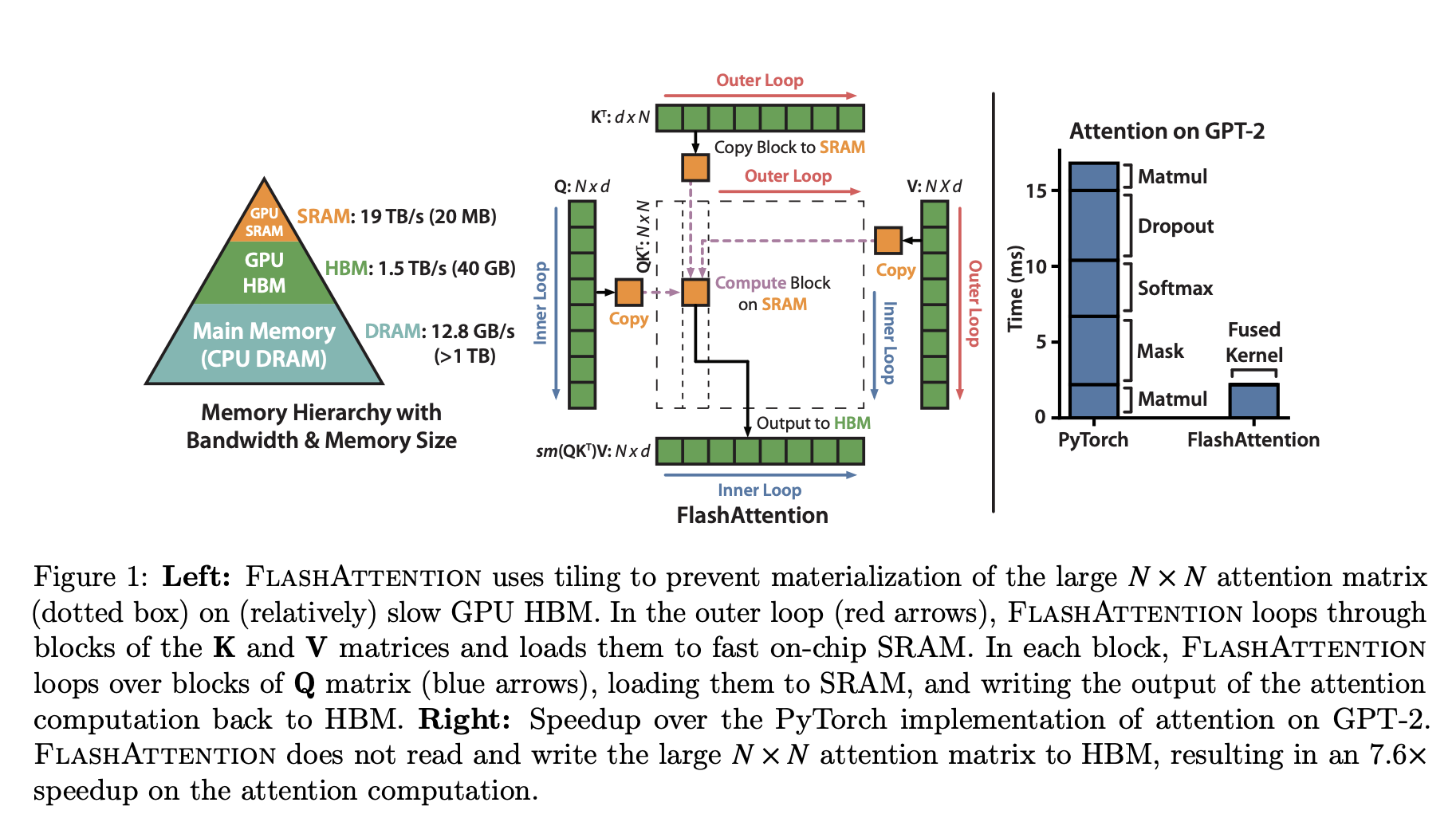 Figure 1 from the FlashAttention paper.
NOTE: this post is about the original FlashAttention paper. There are now three versions of FlashAttention, but we’ll stick with V1 for simplicity.
Tiling
The computation is broken into blocks. The matrices $Q, K, V$ are partitioned into smaller sub-matrices. The algorithm iterates through blocks of $K$ and $V$, loading them into SRAM. Within this outer loop, it iterates through blocks of $Q$.
A simplified view of the loops:
// O is the final output matrix, initialized to zero
// l, m are statistics for the online softmax, initialized
for each block K_j, V_j in K, V:
  Load K_j, V_j into fast SRAM
  for each block Q_i in Q:
    Load Q_i, O_i, l_i, m_i into fast SRAM
    // Core computation, all on-chip
    Compute S_ij = Q_i @ K_j^T
    Compute P_ij = softmax(S_ij) // (This is a simplification, see next section)
    Compute O_ij = P_ij @ V_j
    // Update the output block O_i with the new result
    Update O_i using O_ij and softmax statistics
    // Write the updated O_i, l_i, m_i back to HBM
    Write O_i, l_i, m_i to HBM
This tiled structure changes the memory access pattern. The algorithm iterates through $K$ and $V$ in blocks, reading each element from HBM only once. The critical part is the inner loop. For each block of $K_j$ loaded into SRAM, the algorithm must iterate through all blocks of $Q$ to compute the corresponding updates to the output. This means the algorithm makes multiple passes over the $Q$ matrix. The number of passes is determined by the number of blocks in $K$, which is $T = N/B$, where $B$ is the block size. Since the on-chip SRAM of size $M$ must hold a block of $K$ (size $B \times d$), the block size $B$ is limited to $O(M/d)$. This leads to $T = O(Nd/M)$ passes. Each pass reads the entirety of $Q$ (and reads/writes blocks of $O$), resulting in HBM traffic of $O(Nd \times T) = O(N^2 d^2 / M)$ bytes. This quantity is substantially smaller than the $O(N^2)$ traffic of standard attention.
Example:
To make this concrete, consider an NVIDIA A100 GPU. Each of its Streaming Multiprocessors has 192KB of SRAM. A single kernel will use a portion of this, let’s assume a working SRAM size of M_bytes = 128KB. If we use bfloat16 precision (2 bytes per number), the effective SRAM size in elements is M = 128 * 1024 / 2 = 65,536 elements. For a typical head dimension d=64, $d^2 = 4096$. The reduction factor in memory accesses is approximately $M/d^2 = 65536 / 4096 = 16$. FlashAttention performs roughly 16 times fewer HBM accesses than the standard implementation. For $d=128$, the factor is $M/d^2 = 65536 / 16384 = 4$.
Online Softmax
The softmax function is applied row-wise. For a row $x_i$ of the attention score matrix $S$, the output is $\text{softmax}(x_i)_j = \frac{e^{x_{ij}}}{\sum_k e^{x_{ik}}}$. The denominator requires a sum over the entire row, which seems to prevent block-wise computation.
The “online softmax” algorithm solves this. It computes the exact softmax by maintaining two running statistics for each row $i$: the maximum value seen so far ($m_i$) and the sum of the exponentials of the scaled values ($l_i$). For numerical stability, softmax is computed as:
\[m(x) = \max_j(x_j), \quad l(x) = \sum_j e^{x_j - m(x)}, \quad \text{softmax}(x)_j = \frac{e^{x_j - m(x)}}{l(x)}\]When processing the $j$-th block of a row $x_i$, which we denote $x_{i,j}$, we can update the statistics and the output $O_i$ as follows:
- Compute the local statistics for the current block: $m_{i,j} = \max_k(x_{ik})$ and $l_{i,j} = \sum_k e^{x_{ik} - m_{i,j}}$.
- Compute the new global maximum: $m_i^{\text{new}} = \max(m_i^{\text{old}}, m_{i,j})$.
-
Update the output value using the old and new statistics:
\[O_i^{\text{new}} = \frac{1}{l_i^{\text{new}}} \left( l_i^{\text{old}} e^{m_i^{\text{old}} - m_i^{\text{new}}} O_i^{\text{old}} + l_{i,j} e^{m_{i,j} - m_i^{\text{new}}} O_{i,j} \right)\]where $O_{i,j}$ is the attention output computed using only the current block of $K$ and $V$, and $l_i^{\text{new}}$ is the appropriately rescaled sum.
It’s straightforward to see that by storing and updating these two scalars ($m_i, l_i$) per row, Flash attention can produce the exact output of the softmax operator without needing the whole row at once.
The Backward Pass and Recomputation
The backward pass of attention requires the gradients $\frac{\partial L}{\partial Q}, \frac{\partial L}{\partial K}, \frac{\partial L}{\partial V}$. Computing these requires the matrix $P$ from the forward pass. A standard implementation would read the saved $N \times N$ matrix $P$ from HBM, incurring the same memory bottleneck.
Flash attention avoids this by not storing $P$ at all. Instead, during the backward pass, it recomputes the necessary blocks of the attention matrix $P$ as needed. It does this by loading the required blocks of $Q$, $K$, and $V$ from HBM back into SRAM. The only values saved from the forward pass are the final output $O$ $(N \times d)$ and the online softmax statistics ($m, l$).
This introduces more FLOPs, as parts of the forward pass are re-done. However, since the operation is memory-bound, the time spent on these extra FLOPs is insignificant compared to the time saved by avoiding a massive read from HBM.
Using min cut to determine activation recomputation strategy
Standard automatic differentiation saves many intermediate “activations” from the forward pass to be reused during the backward pass. This can be memory-intensive. Recomputation, or activation checkpointing, is a technique that saves memory by re-calculating these activations during the backward pass instead of storing them. While this suggests a trade-off between memory and compute, a fusing compiler like NVFuser changes the calculation.
For a chain of pointwise operations (e.g., add, relu, cos), a fusing compiler can execute them in a single GPU kernel. The performance of this kernel is limited by memory bandwidth, the speed of reading from and writing to the GPU’s global memory (HBM), not by the arithmetic operations themselves. This means that recomputing a sequence of fused pointwise operations is nearly free, provided the initial input to the sequence is available.
Thus, the problem of choosing which activations to save in the forward pass is about minimizing memory traffic, not necessarily minimizing FLOPs. I came across a very clever strategy for doing this in a blog post by Horace He. There, Horace frames the problem as a “min cut” on the computation graph and sees some nice improvements. I recommend reading the post for details. Here I’ll mainly work out some details that I was confused about in Horace’s original post. 1
Backward and forward passes
Consider the function f(a,b,c,d) = cos(cos(a+b+c+d)). Let z = a+b+c+d. The forward pass computes z, then cos(z), then y = cos(cos(z)).
The chain rule dictates what the backward pass needs. To compute the gradients, it requires the intermediate values, or “activations,” z and cos(z) to calculate sin(z) and sin(cos(z)):
dy             = incoming ∂L/∂y
dcos           = dy * (-sin(x.cos()))
dx             = dcos * (-sin(x))
da,db,dc,dd    = dx
A standard autograd system, as shown in the first figure, would save the z and cos(z), require 2 reads and 2 writes. This ensures the values are available for the backward pass.
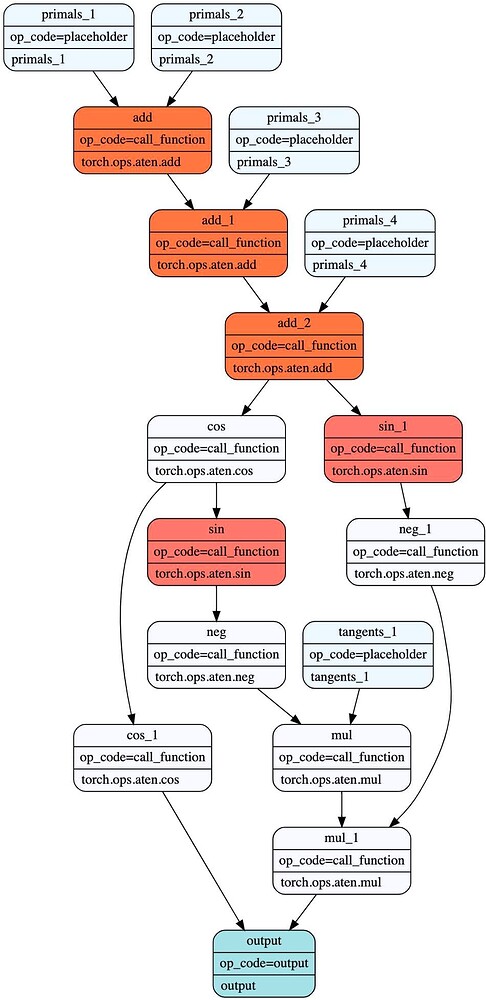
This is a safe but suboptimal strategy. The total data transferred between the forward and backward passes for this strategy is the size of two tensors. We can do better. The key insight is that if we save only z (the output of add_2), we can recompute cos(z) on-the-fly inside the backward pass’s fused kernel. This halves the memory traffic.
The Min-Cut Formulation
To find this optimal set of checkpointed tensors automatically, we model the problem as finding a minimum cut in a graph.
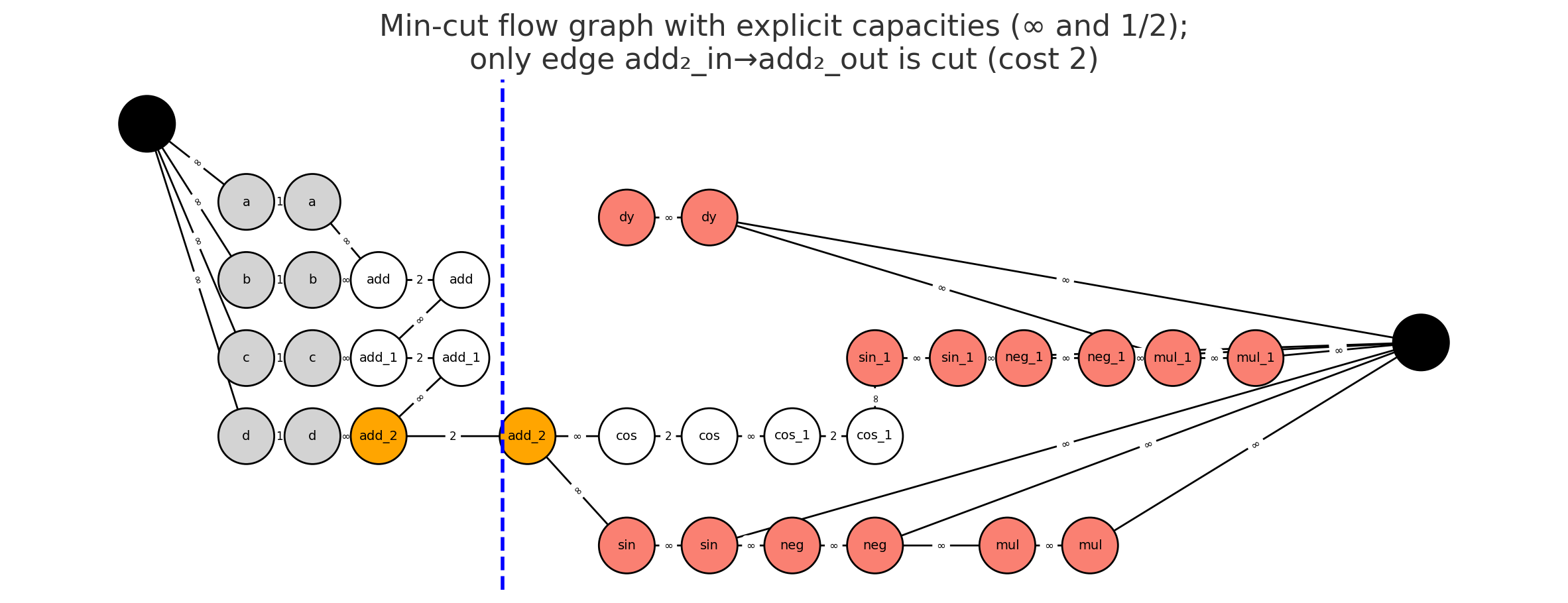
-
The Graph: We construct a graph representing the full forward and backward computation. We add a virtual source,
SRC, and a virtual sink,SNK. - The Source and Sink Sets:
- The source set represents the beginning of the forward pass. The
SRCnode is connected to all initial inputs of the model (e.g.,a, b, c, d). - The sink set represents the operations that must run in the backward pass. An operation must be in the backward pass if it depends on the incoming gradient. This set of operations is called the tangent closure. In the figures, these are the red nodes. The
SNKnode is connected to all nodes in the tangent closure.
- The source set represents the beginning of the forward pass. The
-
Edges and Costs: The problem is transformed into a standard edge-cut problem via node splitting. Every operation node
vis split into two nodes,v_inandv_out, connected by an edge.- Split Edges (
v_in -> v_out): These are the only edges with a finite cost, or. The cost of this edge is the cost of checkpointing the tensorv.Cost = 2 * B(v)for an intermediate activation. This cost represents onewriteto global memory and onereadfrom it.Cost = 1 * B(v)for a forward pass input that already exists in global memory. This cost represents just oneread. Here,B(v)is the size of the tensor in bytes.
- Data-Flow Edges (
u_out -> v_in): Edges representing the flow of data between operations have infinite cost. This models our assumption that recomputation within a fused kernel is free.
- Split Edges (
-
The Cut: The min-cut algorithm finds the set of edges with the minimum total cost that must be severed to separate
SRCfromSNK. Because only the split edges have finite cost, the algorithm will only sever those.Mathematically, the algorithm solves for the
\[\text{minimize} \sum_{(u \to v) \in \text{cut}} \text{cost}(u \to v)\]s-tcut 2 with minimum total cost:The sum is over all edges in the cut. Since data-flow edges have infinite cost, a minimal cut will only ever consist of the finite cost”split edges.” The problem is thus equivalent to finding the cheapest set of split edges to sever.
An edge
v_in -> v_outbeing cut means we have decided to pay its cost and checkpoint the tensorv. The nodes whose edges are cut are colored orange. Nodes on theSRCside of the cut are inputs. Nodes on theSNKside are either part of the mandatory tangent closure (red) or are operations that will be recomputed (white).
For our example, the algorithm compares the costs of all possible cuts:
- Cut at
add_2: Severs theadd_2_in -> add_2_outedge. Cost =2B. - Cut at
cosandcos_1: Severs two edges. Cost =2B + 2B = 4B. - Cut at the inputs: Severs four edges. Cost =
1B + 1B + 1B + 1B = 4B.
The minimum cost is 2B, corresponding to cutting only the add_2 edge. This means the optimal strategy is to checkpoint add_2 (orange), recompute cos and cos_1 (white), and feed the results to the tangent closure (red).
Thus, the min-cut formulation finds the checkpointing strategy that minimizes memory traffic under the fused computation model. These min-cut problems can be solved efficiently with standard max-flow algorithms.
-
See also this paper, which Horace pointed me to. ↩
-
An
s-tcut is a set of edges whose removal disconnects all paths fromSRCtoSNK. ↩
Linear layouts, triton, and linear algebra over F_2
@typedfemale posted the paper “Linear Layouts: Robust Code Generation of Efficient Tensor Computation Using F2” on X (link to tweet). It looked interesting. I tweeted:
“I will actually read this. it’s always the very interesting things that use lin alg over finite fields. i remember in undergrad when i first saw a “real” application of it while learning the general number field sieve.”
I struggled with this paper. This post is the result of that effort. Hopefully, it is useful.
My goal here is to just give a sense of their main idea: using linear algebra over the finite field $F_2$ to manage how tensor data is arranged for computation on GPUs. This is outside my usual area of optimization and machine learning, but anyway it looked like a fun read.
1. GPU and Tensor Layouts
Deep learning models use many tensor computations. GPUs accelerate these computations. The specific arrangement of tensor data on the GPU is called a “tensor layout.” This layout dictates, for example, which register within a specific thread (itself part of a GPU warp, a group of threads executing in lockstep) holds which piece of tensor data for an operation. This layout directly affects performance.
Current methods for defining and managing tensor layouts can apparently be complex.1 They can be specific to particular hardware or operations. This makes it difficult to build systems that are both flexible for different models and hardware, and also consistently fast and error-free. Incorrect or inefficient layouts lead to slow memory access, underused compute units, and slower models.
Triton is a language and compiler, originally developed by OpenAI, for writing custom code segments that run on GPUs, known as GPU kernels. People who train like to write performant ML code use Triton to create these kernels, for example, to fuse multiple operations (like a matrix multiplication followed by an activation function) into a single GPU kernel. The “Linear Layouts” paper aims to improve how Triton’s compiler system handles these tensor layouts.
2. Linear Layouts via Linear Algebra over $\mathbb{F}_2$
The paper “Linear Layouts: Robust Code Generation of Efficient Tensor Computation Using $\mathbb{F}_2$” defines a tensor layout using linear algebra over the finite field $\mathbb{F}_2 = \{0, 1\}$. Each layout is a matrix $A$ with entries in $\mathbb{F}_2$. This matrix $A$ specifies a linear map.
For a distributed layout, this map assigns tensor data to specific hardware processing units and their local storage. The matrix $A$ maps an identifier for a hardware resource to the coordinates of a logical tensor element.
- The input to this map (the domain) is a vector $v \in \mathbb{F}_2^n$. The bits of $v$ identify a unique hardware slot. This vector is a concatenation of bit vectors representing, for example, a register index $v_{\text{reg}}$, a thread index $v_{\text{thr}}$, and a warp index $v_{\text{wrp}}$, so $v = [v_{\text{reg}} | v_{\text{thr}} | v_{\text{wrp}}]$.
- The output of the map (the codomain) is a vector $w \in \mathbb{F}_2^m$. The bits of $w$ are the binary representation of the coordinates of an element in the logical tensor. For a 2D tensor
Tensor[i,j], $w$ would be formed by concatenating the binary representations of the integer indices $i$ and $j$, e.g., $w = [\text{bits}(i) | \text{bits}(j)]$. - The mapping is $w = Av$. All matrix and vector operations use $\mathbb{F}_2$ arithmetic, where addition is XOR and multiplication is AND.
This matrix $A$ dictates which hardware slot $v$ is responsible for which logical tensor element $w$. The authors state this system can represent existing layouts, such as those in Triton, and define new ones because these mappings from hardware bit identifiers to logical coordinate bit identifiers can be expressed as such matrices.
Example: Layout A from Figure 1 (Page 4 of the Paper)
Figure 1a in the paper illustrates two distributed layouts.
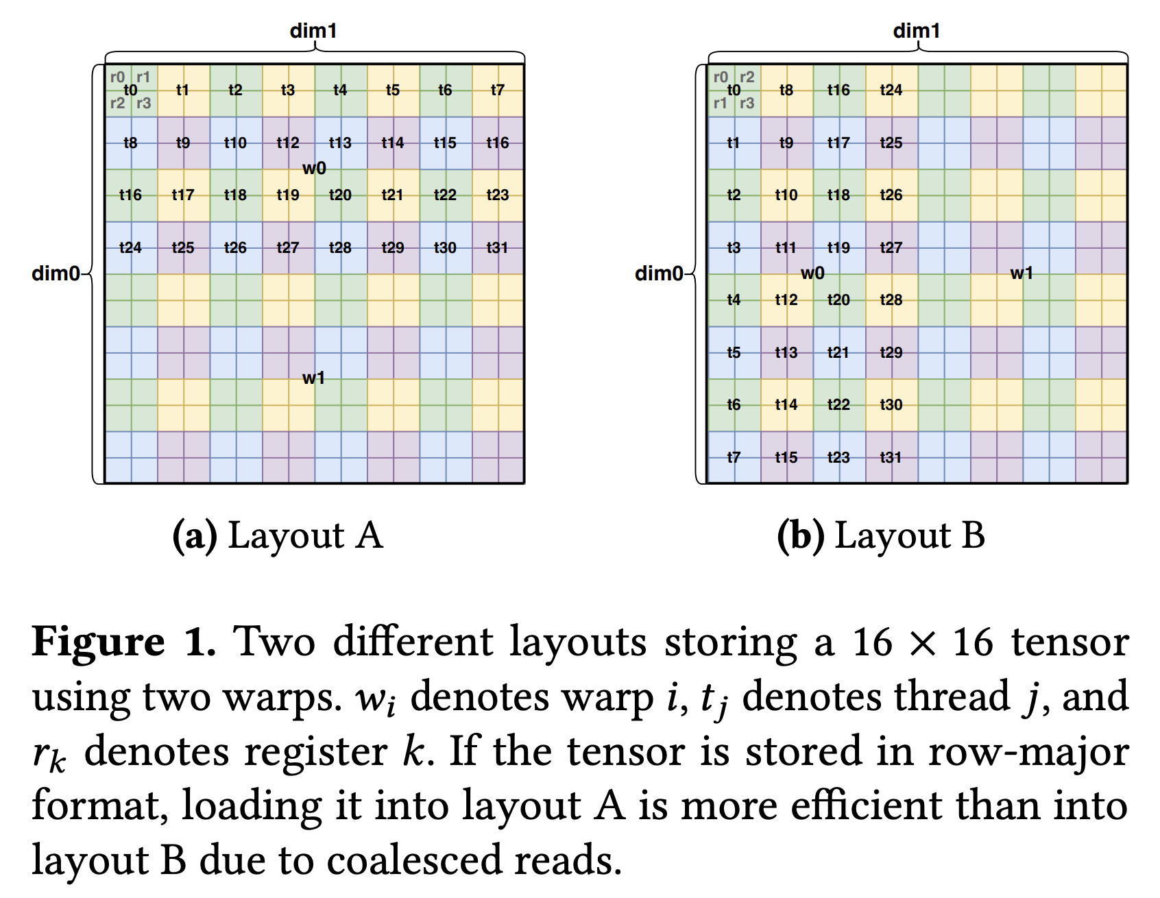
Let’s look into Layout A, which can be represented by a $8 \times 8$ matrix $A$ with entries in $\mathbb{F}_2$. This matrix maps an 8-bit hardware ID $v$ to an 8-bit logical coordinate $w$ for a $16 \times 16$ tensor.
-
Input:
\[v = [v_0(\text{reg}_0) \, v_1(\text{reg}_1) \,|\, v_2(\text{thr}_0) \, v_3(\text{thr}_1) \, v_4(\text{thr}_2) \, v_5(\text{thr}_3) \, v_6(\text{thr}_4) \,|\, v_7(\text{wrp}_0)]^T\](Bit $v_k$ is the $k$-th component of $v$; labels like $\text{reg}_0$ indicate conceptual roles).
-
Output:
\[w = [w_0(i_0) \, w_1(i_1) \, w_2(i_2) \, w_3(i_3)\, |\, w_4(j_0) \, w_5(j_1) \, w_6(j_2) \, w_7(j_3) ]^T\]The bits $w_0..w_3$ form the column index $j$ ($j_0$ is LSB). The bits $w_4..w_7$ form the row index $i$ ($i_0$ is LSB).
Note we’re slightly deviating from the paper. There, they define $w_{0:3} = j$ and $w_{4:7} = i$. I find it more natural to define $w_{0:3} = i$ and $w_{4:7} = j$. This means that $j = w_7\cdot 2^3 + w_6 \cdot 2^2 + w_5\cdot 2^1 + w_4\cdot 2^0$, etc
To construct the matrix $A$ frin Figure 1a for this linear layout, we observe that it’s mapping $w = Av$ has the following effect.
- Incrementing $v_0$ (respectively, $v_1$) increments $j$ by $1$ (respectively, $i$ by $1$). Thus, the least significant bit $w_4$ of $j$ (respectively $w_0$ of $i$) is precisely $v_0$ (respectively $v_1$).
- Incrementing $v_2$ increments $j$ by $2$. Thus, the second bit $w_5$ of $j$ is precisely $v_2$. Likewise, incrementing $v_5$ by $1$ increments $i$ by $2$, so the second bit $w_2$ of $i$ is precisely $v_5$.
Continuing with similar reasoning, we can show the following:
\[A = \begin{pmatrix} % v0 v1 v2 v3 v4 v5 v6 v7 0 & 1 & 0 & 0 & 0 & 0 & 0 & 0 \\ % w0 (i0) 0 & 0 & 0 & 0 & 0 & 1 & 0 & 0 \\ % w1 (i1) 0 & 0 & 0 & 0 & 0 & 0 & 1 & 0 \\ % w2 (i2) 0 & 0 & 0 & 0 & 0 & 0 & 0 & 1 \\ % w3 (i3) 1 & 0 & 0 & 0 & 0 & 0 & 0 & 0 \\ % w4 (j0) 0 & 0 & 1 & 0 & 0 & 0 & 0 & 0 \\ % w5 (j1) 0 & 0 & 0 & 1 & 0 & 0 & 0 & 0 \\ % w6 (j2) 0 & 0 & 0 & 0 & 1 & 0 & 0 & 0 % w7 (j3) \end{pmatrix}\]From this matrix, you can verify that it indeed maps various hardware ids slots to the correct logical tensor elements. For example, the slot with the slot corresponding to register 0, thread 0, warp 0 maps to the logical tensor element Tensor[0,0], $i = w_{3:0} = 0000$ and $j = w_{7:4} = 0000$ (notice I reversed the bits). On other hand, the slot corresponding to register 1, thread 1, warp 0 maps to the logical tensor element Tensor[0,3], $i = w_{3:0} = 0000$ and $j = w_{7:4} = 0011$.
3. Memory Layouts and Shared Memory Interaction
Distributed layouts assign tensor elements to hardware compute units. Memory layouts describe how these logical tensor elements are arranged linearly within a memory segment, such as a GPU’s global or shared memory. A memory layout can be represented by a matrix $M_{\text{mem}}$ with entries in $\mathbb{F}_2$. This matrix $M_{\text{mem}}$ maps a vector representing a memory offset to the bits of the logical tensor coordinate stored at that offset:
logical_tensor_coordinate = M_mem * memory_offset_bits.
When we know the logical coordinate of a tensor element and need to find its location in memory, we use the inverse map, $M_{\text{mem_inv}}$. This matrix maps the bits of a logical tensor coordinate to the bits of its memory offset:
memory_offset_bits = M_mem_inv * logical_tensor_coordinate_bits.
A Simple Memory Layout: Row-Major Order
To understand memory access patterns, we first consider a basic row-major arrangement for a $16 \times 16$ tensor, Tensor[i,j]. The linear memory offset is offset = i * 16 + j (assuming unit-sized elements). Suppose the logical coordinate vector $w$ follows our convention: $w = [w_0(i_0) \dots w_3(i_3) | w_4(j_0) \dots w_7(j_3)]^T$. Here, $w_{0..3}$ are the bits of $i$ (LSB $i_0$ to MSB $i_3$), and $w_{4..7}$ are the bits of $j$ (LSB $j_0$ to MSB $j_3$). The memory offset $k$ is an 8-bit value $k = [k_0(\text{MSB}) \dots k_7(\text{LSB})]^T$. For row-major storage, the column index $j$ forms the lower-order bits of the offset ($k_{0..3}$), and the row index $i$ forms the higher-order bits ($k_{4..7}$).
The matrix $M_{\text{mem_inv}}: w \mapsto k$ that achieves this is an $8 \times 8$ permutation matrix:
This matrix $M_{\text{mem_inv}}$ takes $w=[\text{bits}(i) | \text{bits}(j)]$ and produces $k=[\text{bits}(j) | \text{bits}(i)]$, correctly placing $j$-bits into the lower part of $k$ and $i$-bits into the higher part.
GPU Shared Memory Structure
A GPU’s shared memory is a fast, on-chip memory. It is physically divided into multiple (e.g., 32) independent banks. Each bank contains many addressable lines (also called vector words or cache lines), typically the size of a wide hardware memory access (e.g., 128 bits). Each line stores multiple individual data elements (e.g., four 32-bit floats).
A specific data element within shared memory is pinpointed by three components:
bank_hw: Selects the physical bank.idx_hw: Selects the line (vector word) within that bank.vec_hw: Selects the specific element within that chosen line.
A useful way to visualize this memory is:
bank 0: [line 0, line 1, line 2, ..., line N-1]
bank 1: [line 0, line 1, line 2, ..., line N-1]
...
bank 31: [line 0, line 1, line 2, ..., line N-1]
Accessing different banks simultaneously is done in parallel (to my knowledge). Accessing the same bank simultaneously by different threads for different lines causes bank conflicts, serializing operations. On the other hand, accessing elements within the same line simultaneously can be performed in parallel; this is called vectorized access. Efficient memory access thus requires careful mapping of data to these (vec_hw, bank_hw, idx_hw) components.
The Swizzling Map s
The paper’s “optimal swizzling” algorithm constructs a specialized memory layout for shared memory, defined by an $\mathbb{F}_2$ matrix $s$. This map $s$ defines how the structured shared memory hardware components map to the logical tensor coordinate stored at that physical slot:
- Input (domain): A bit vector
v_sm = [vec_hw | idx_hw | bank_hw]representing a shared memory slot description. - Output (codomain): The logical tensor coordinate $w = [\text{bits}(i) | \text{bits}(j)]$ (using our convention for $w$) stored at that slot.
- Mapping: $w = s \cdot v_{\text{sm}}$.
The purpose of constructing this swizzling map $s$ is to arrange logical data across physical shared memory slots in a non-obvious (“swizzled”) manner. This design ensures that when threads (operating under a given distributed layout) need to access various logical tensor coordinates, the corresponding shared memory hardware slots (vec_hw, idx_hw, bank_hw) (found via $s^{-1}(w)$) are distributed to minimize bank conflicts and enable efficient vectorized reads and writes.
4. Linear Algebra and Layouts
A compiler must perform several tasks to generate efficient GPU code: it must arrange data for memory access, rearrange it for computation, and map these operations to specialized hardware instructions. Representing layouts as matrices allows the compiler to perform these tasks using linear algebra.
Layout Conversion Between Layouts Optimized for Memory and Compute
We can use matrix products to represent how a GPU kernel moves data between a layout optimized for memory access and one required by a compute unit.
Loading data from global memory is fastest when threads access contiguous blocks of memory, a pattern known as coalesced access. This suggests a simple, row-major layout. However, a specialized compute unit, like a Tensor Core, may require data to be presented in a completely different layout to perform its calculations. We can compute this conversion using matrix products.
Let layout $A$ be the source (e.g., memory layout) and $B$ be the destination (e.g., compute layout). We need to find the transformation $C$ that maps a hardware resource $v_A$ in the source layout to its corresponding resource $v_B$ in the destination. The same logical data $w$ must satisfy $w = Av_A$ and $w = Bv_B$.
For layout $B$ to be a valid destination, it must be surjective, i.e., its mapping can reach every element of the logical tensor. This guarantees that a right inverse $B^{-1}$ exists. By setting the expressions for $w$ equal, we find the conversion map:
\[v_B = (B^{-1}A)v_A\]The structure of the resulting matrix $C = B^{-1}A$ describes the hardware operations needed to move data. For example, if $C$ only permutes register bits, the conversion is a simple move between registers within each thread. If it mixes bits between different threads within a warp, it requires an “intra-warp shuffle,” a hardware instruction that exchanges data between threads in the same execution group.
Product Operator for Hierarchical Layout Design
The product operator constructs complex layouts from simpler component layouts. This process corresponds to creating a block-diagonal matrix. A developer can define a layout for registers within a thread ($L_{reg}$) and a layout for the threads in a warp ($L_{thr}$) separately. The product operator $L_{reg} \times L_{thr}$ combines them into a single layout $L$ for the entire warp. The matrix for $L$ is the block-diagonal composition of its component matrices:
\[L = \begin{pmatrix} L_{reg} & 0 \\ 0 & L_{thr} \end{pmatrix}\]Left Division for Matching Hardware Instructions
Left division determines if a data layout can be loaded or stored using a specialized hardware instruction. An instruction like ldmatrix loads a fixed-size tile of data from shared memory into registers. Its operation is defined by a corresponding tile layout, a small matrix $T$. This matrix maps the hardware resources for a single instruction call (e.g., the bits of the register IDs) to the data it acts upon (e.g., the bits of the memory offsets).
The compiler checks if the kernel’s larger data layout $L$ is compatible with the instruction’s tile layout $T$. This is not arithmetic division. It is a test of matrix structure. Left division $L / T$ succeeds if $L$ can be decomposed into the block-diagonal form:
\[L = \begin{pmatrix} T & 0 \\ 0 & R \end{pmatrix}\]where $R$ is the remainder layout. This decomposition confirms that a subset of $L$’s input resources maps to a subset of its output data using a transformation that is structurally identical to $T$, with no interference from the other resources governed by $R$.
If the division succeeds, the compiler can generate a sequence of ldmatrix instructions to load the data for the entire layout $L$. The tile layout $T$ governs the loading of the first block. The remainder layout $R$ is then used to calculate the starting address for the next block, and the process is repeated. This automates the use of high-throughput hardware instructions for any compatible layout.
Unification of Triton’s Layouts
In Triton’s legacy system, conversions between different layout types led to a “quadratic explosion” of custom implementations. Each pair of layouts required a unique, manually-coded conversion function. This made the compiler complex and difficult to extend, as adding a new layout type required implementing new conversion paths to all existing types.
The paper proves that all of Triton’s legacy layouts can be represented as linear layouts (Theorem 4.9). This result allows the compiler to replace the entire system of custom conversion functions with a single matrix operation. The conversion from any layout $A$ to any layout $B$ is now specified by the matrix product $B^{-1} A$.
This simplifies compiler development. To add a new layout, a developer provides its matrix definition. Conversions to and from all other defined layouts are then handled by the existing matrix product operation.
5. Optimizing Code
The framework allows a compiler to automate optimizations by translating them into questions about matrix properties.
Vectorization
Previously, Triton identified vectorization opportunities by finding a tensor’s fastest-running dimension and assuming it determined contiguity. This heuristic fails for a tensor of shape [128, 1]. The fastest-running dimension has size 1, so Triton would disable vectorization, even though 128 contiguous elements are available along the other dimension.
The linear layout method replaces this inference with a direct computation. The physical property of contiguous logical elements being stored in contiguous registers is equivalent to an identity map on their address bits.
More specifically, the compiler queries the layout’s inverse matrix, $L^{-1}$. It finds the largest integer $k$ for which the $k \times k$ sub-matrix mapping the lowest-order logical bits to the lowest-order register bits is the identity matrix. This $k$ is the precise vectorization width, calculated directly from the layout’s structure.
Broadcasting
Broadcasting is the replication of a single logical element across multiple hardware resources, such as different threads. In a reduction operation, like a sum, these duplicated values must be counted only once to avoid incorrect results.
Linear layouts provide a direct method for identifying this replication. Specifically, the duplication of a logical element across threads is represented in the layout matrix $A$ as a zero-column in the section corresponding to the thread ID bits.
A zero-column means that changing the thread ID does not change the resulting logical address $w$ in the mapping $w = Av$. The compiler inspects the matrix for this property to ensure each logical element is processed only once during a reduction.
Mixed-Precision Data Shuffling
A mixed-precision matrix multiplication computes the product of two matrices with different data types, such as mxfp4 and bf16. The overall computation is tiled, meaning it is broken down into smaller matrix multiplications on tiles of the input data. A performance bottleneck arises if the bf16 tiles cannot be loaded into registers as efficiently as the mxfp4 tiles.
The GPU hardware can execute wide vector instructions, which load a fixed-size block of data (e.g., 16 bytes) from a contiguous block of memory addresses in a single operation. The challenge is to arrange the data in memory such that all elements needed for a single compute tile are physically contiguous and can be fetched with one of these instructions.
For the bf16 data type, a standard memory layout may not have this property. The solution is a data shuffle: a pre-processing step that copies the bf16 data into a new arrangement within on-chip shared memory, organizing it so that each tile’s worth of data resides in a contiguous block of addresses.
The user specifies the logic of this shuffle with a high-level shape operation. For instance, if the hardware instruction expects a tile’s data in a layout that is logically the transpose of what a simple load provides, the user specifies a tt.transpose operation.
This shape operation is a linear transformation on the tensor’s logical coordinates and is represented by a permutation matrix, $T_{shape}$. The compiler combines this with the original layout matrix, $A_{bf16}$, to compute the new, shuffled layout $A_{shuffled}$:
\[A_{shuffled} = T_{shape}A_{bf16}\]The compiler uses this resulting matrix $A_{shuffled}$ to generate the code that performs the physical memory copy for the shuffle.
Generating Code for Layout Conversions
To convert a tensor from a source distributed layout $A$ to a destination distributed layout $B$, the compiler first computes the conversion matrix $C = B^{-1}A$. This matrix maps the source hardware resources to the destination hardware resources. The structure of $C$ determines the cheapest hardware primitive that can perform the conversion.
The compiler checks the structure of $C$ in order of cost, from cheapest to most expensive.
-
Intra-thread Register Move: This is the cheapest conversion. It is possible if the data movement is confined entirely within each thread. This is the case if the conversion matrix $C$ only permutes register bits, meaning the sub-matrix $(B^{-1}A)_{reg}$ is a permutation matrix and the rest of $C$ is the identity.
-
Intra-warp Shuffle: If an intra-thread move is not possible, the compiler checks if the conversion can be done with warp shuffles. A warp shuffle is a hardware instruction that allows threads within the same warp to exchange data directly without using shared memory. This is possible if the conversion matrix $C$ does not move data between warps, which corresponds to the warp-related block of the matrix, $(B^{-1}A)_{wrp}$, being the identity matrix.
-
Inter-warp Conversion via Shared Memory: If neither of the above conditions is met, data must move between different warps. This is the most expensive conversion and requires using on-chip shared memory as an intermediary. Data from the source warps is written to shared memory and then read by the destination warps.
Generating Warp Shuffles
When a conversion requires an intra-warp data exchange, the compiler generates a sequence of hardware shfl.sync instructions. A receiving thread executes shfl.sync(value, srcLane) to fetch a value from the registers of a sending thread, identified by its lane index srcLane. The linear layout framework provides a direct method for calculating these parameters.
This process is illustrated by the example in Figure 3.
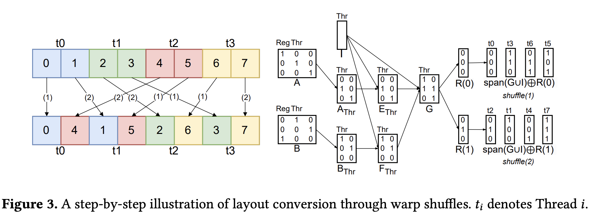 Figure 3: Layout conversion via warp shuffles from the paper. The labels
 t_i denote 3-bit logical address vectors. Note that the t0,..,t7 in the top right corner are not threads, they are just labels for the basis vectors.
1. Determine the Exchange Vector ($V$)
First, the compiler identifies data that can be moved as a single vector. This data corresponds to the intersection of the register-related column subspaces, $A_{reg} \cap B_{reg}$. Any data in this subspace maintains its relative position within the registers during the conversion.
Because this block of data is structurally invariant, it can be moved as a single unit. The compiler selects a basis $V$ for the largest possible subspace within this intersection whose total data size does not exceed the hardware’s 32-bit shfl.sync payload limit. This basis $V$ defines the vector that will be moved in each shuffle instruction.
2. Decompose the Address Space
The compiler creates a plan by decomposing the logical address space, which combines register and thread addresses. It computes bases for several subspaces.
- $I = \text{span}(A_{thr}) \cap \text{span}(B_{thr})$: Data that does not move between threads.
- $E = A_{thr} \setminus I$ and $F = B_{thr} \setminus I$: Subspaces of data to be sent and received.
- $G = {e_i \oplus f_i}$: The set of displacement vectors. The paper specifies that $G$ is constructed “After choosing an ordering for $E$ and $F$.” This implies a one-to-one pairing $(e_i, f_i)$ based on the chosen ordering of the basis vectors. This pairing is necessary because the conversion is a permutation: each source data element $e_i$ has a unique destination $f_i$.
- $R$: A basis for the intra-thread (register) address space. This is a basis for the complement of the thread space not already covered by the vectorized subspace $V$, $\text{span}(A_{thr} \cup B_{thr} \cup V)$.
3. Sequence the Exchange
A thread holds more data than one shuffle can move. The exchange is thus partitioned into rounds, one for each basis vector in $R$. A larger vectorization $V$ results in a smaller basis $R$ and fewer rounds.
In Figure 3, $V$ is empty, $R$ has two vectors, $R(0)$ and $R(1)$, corresponding to the two data elements held by each thread.
- Round 1 (
shuffle(1)): This round moves the data slice whose logical addresses are in the affine subspace $\text{span}(G \cup I) \oplus R(0)$. A single data element’s logical address is $e_i \oplus R(0)$.valueparameter: Thevalueis the vector defined by $V$ from the register slice selected by $R(0)$.srcLaneparameter: A receiving thread at a destination thread address $f_i$ uses its corresponding displacement $g_i$ to find its source thread address $e_i = f_i \oplus g_i$. The integer representation of this vector $e_i$ is used as thesrcLane.
- Round 2 (
shuffle(2)): This round moves the data slice corresponding to the second register, selected by $R(1)$. The logical addresses are $\text{span}(G \cup I) \oplus R(1)$. Thevalueis now the data from the second register slice, but thesrcLanefor each thread is calculated using the same exchange pattern $G$ as in the first round.
Running Out of Steam
There is a bunch of other cool stuff in the paper. I ideally wanted to present “optimal swizzling,” but I timeboxed this post, and so I think I’ll end it here.
-
From what I can understand. I am not a GPU expert, but I will write like I am one for the purpose of this post. ↩
Modded-NanoGPT Walkthrough II: Muon Optimizer, Model Architecture, and Parallelism
In Part I of this walkthrough, we covered the initial setup, compiler configurations, and custom FP8 operations within the modded-nanogpt repository’s train_gpt.py script. This second part continues the walkthrough of train_gpt.py. We will look at the Muon optimizer, GPT model architecture, and the distributed training strategies.
Table of Contents
- The Muon Optimizer: Iterative Orthogonalization for Updates
- GPT Model Architecture: Component Details
- Parallelism and Distributed Training
The Muon Optimizer: Iterative Orthogonalization for Updates
The train_gpt.py script introduces a custom optimizer called Muon, that is specifically used with the matrix layers of the transformer model. (For the nonmatrix layers, they use an Adam method.) In short, Muon replaces the matrix blocks of the gradient1 with a new matrix with better conditioning and the same row/column space. This is achieved by applying an iterative algorithm called the Newton-Schulz.
Why do they do this? From my read of the literature (up to June 02, 2025), there has been no strong theoretical justification for doing so. Although we can realize it as a variant of gradient descent in a block spectral norm, we don’t know why it’s good to do gradient descent in the spectral norm for transformer models. 🤷
A. zeropower_via_newtonschulz5: Orthogonalizating the gradient
The function zeropower_via_newtonschulz5 applies Newton-Schulz to an input matrix $G$. Classically, the method was designed to do the following:
If $G$ has a singular value decomposition (SVD) $G = U \Sigma V^T$, this iteration (when properly initialized) converges quadratically to a matrix $G’ \approx U I’ V^T$. In this expression, $I’$ is a diagonal matrix with entries of 1 where $\Sigma$ had non-zero singular values, and 0 otherwise. This process yields an (approximately) orthogonal matrix with the same row and column space as $G$.
The method in the code is slightly different. It instead modifies the iteration so that the singular values near zero become larger more quickly, but the limiting singular values (empirically) reach the interval between .5 and 1.5. This seems to work OK.
@torch.compile
def zeropower_via_newtonschulz5(G: Tensor, steps: int) -> Tensor:
    """
    Newton-Schulz iteration to compute the zeroth power / orthogonalization of G. We opt to use a
    quintic iteration whose coefficients are selected to maximize the slope at zero. For the purpose
    of minimizing steps, it turns out to be empirically effective to keep increasing the slope at
    zero even beyond the point where the iteration no longer converges all the way to one everywhere
    on the interval. This iteration therefore does not produce UV^T but rather something like US'V^T
    where S' is diagonal with S_{ii}' ~ Uniform(0.5, 1.5), which turns out not to hurt model
    performance at all relative to UV^T, where USV^T = G is the SVD.
    """
    assert G.ndim >= 2 # batched Muon implementation by @scottjmaddox, and put into practice in the record by @YouJiacheng
    a, b, c = (3.4445, -4.7750,  2.0315)
    X = G.bfloat16()
    if G.size(-2) > G.size(-1):
        X = X.mT

    # Ensure spectral norm is at most 1
    X = X / (X.norm(dim=(-2, -1), keepdim=True) + 1e-7)
    # Perform the NS iterations
    for _ in range(steps):
        A = X @ X.mT
        B = b * A + c * A @ A # quintic computation strategy adapted from suggestion by @jxbz, @leloykun, and @YouJiacheng
        X = a * X + B @ X

    if G.size(-2) > G.size(-1):
        X = X.mT
    return X
Walking through the code, the operations are as follows: The input tensor G, representing a gradient update, is first cast to bfloat16 precision. If the input matrix G has more rows (G.size(-2)) than columns (G.size(-1)), it is transposed. Let X be this potentially transposed matrix. The iteration then computes A = X @ X.mT. The dimensions of A are X.size(-2) x X.size(-2). The initial transposition ensures X.size(-2) is the smaller of G’s original two dimensions. This makes the intermediate matrix A (and subsequent products like A@A) smaller, reducing computational cost.
Next, X is normalized by its spectral norm. The code approximates this using X.norm(dim=(-2, -1), keepdim=True), and adds a small epsilon 1e-7 for numerical stability. This normalization puts $X$ into the region of quadratic convergence for the (classical) Newton-Schulz iteration.
The core of the function is the iterative application of a quintic formula:
\[X_{k+1} = a X_k + (b(X_k X_k^T) + c(X_k X_k^T)^2) X_k\]The constants $a, b, c$ are (3.4445, -4.7750, 2.0315). This iteration runs for a specified number of steps (the default ns_steps for Muon is 52). Finally, if X was initially transposed, it is transposed back. The @torch.compile decorator is used to optimize this function into efficient GPU kernels.
B. The Muon Optimizer Class
The Muon class, defined by inheriting from torch.optim.Optimizer, implements the custom update rule for 2D matrix parameters.
class Muon(torch.optim.Optimizer):
    """
    Muon - MomentUm Orthogonalized by Newton-schulz

    https://kellerjordan.github.io/posts/muon/

    Muon internally runs standard SGD-momentum, and then performs an orthogonalization post-
    processing step, in which each 2D parameter's update is replaced with the nearest orthogonal
    matrix. To efficiently orthogonalize each update, we use a Newton-Schulz iteration, which has
    the advantage that it can be stably run in bfloat16 on the GPU.

    Some warnings:
    - This optimizer should not be used for the embedding layer, the final fully connected layer,
    or any {0,1}-D parameters; those should all be optimized by a standard method (e.g., AdamW).
    - To use it with 4D convolutional filters, it works well to just flatten their last 3 dimensions.

    Arguments:
        lr: The learning rate used by the internal SGD.
        momentum: The momentum used by the internal SGD.
        nesterov: Whether to use Nesterov-style momentum in the internal SGD. (recommended)
        ns_steps: The number of Newton-Schulz iteration steps to use.
    """
    def __init__(self, params, lr=0.02, momentum=0.95, nesterov=True, ns_steps=5, rank=0, world_size=1):
        self.rank = rank
        self.world_size = world_size
        defaults = dict(lr=lr, momentum=momentum, nesterov=nesterov, ns_steps=ns_steps)
        params: list[Tensor] = [*params]
        param_groups = []
        for size in {p.numel() for p in params}:
            b = torch.empty(world_size, size, dtype=torch.bfloat16, device="cuda")
            group = dict(params=[p for p in params if p.numel() == size],
                         update_buffer=b, update_buffer_views=[b[i] for i in range(world_size)])
            param_groups.append(group)
        super().__init__(param_groups, defaults)

    @torch.no_grad()
    def step(self):
        for group in self.param_groups:
            update_buffer: Tensor = group["update_buffer"]
            update_buffer_views: list[Tensor] = group["update_buffer_views"]
            params: list[Tensor] = group["params"]
            handle = None
            params_world = None
            def update_prev(): # optimized Muon implementation contributed by @YouJiacheng
                handle.wait()
                for p_world, g_world in zip(params_world, update_buffer_views):
                    p_world.add_(g_world.view_as(p_world),
                                 alpha=-group["lr"] * max(1, p_world.size(-2) / p_world.size(-1))**0.5)
            for base_i in range(len(params))[::self.world_size]:
                if base_i + self.rank < len(params):
                    p = params[base_i + self.rank]
                    g = p.grad
                    assert g is not None
                    state = self.state[p]
                    if "momentum_buffer" not in state:
                        state["momentum_buffer"] = torch.zeros_like(g)
                    buf: Tensor = state["momentum_buffer"]
                    buf.lerp_(g, 1 - group["momentum"])
                    g = g.lerp_(buf, group["momentum"]) if group["nesterov"] else buf
                    g = zeropower_via_newtonschulz5(g, steps=group["ns_steps"]).flatten()
                else:
                    g = update_buffer_views[self.rank]
                if base_i > 0:
                    update_prev()
                handle = dist.all_gather_into_tensor(update_buffer, g, async_op=True)
                params_world = params[base_i : base_i + self.world_size]
            update_prev()
The __init__ method groups parameters by their total number of elements (p.numel()). For each unique element count (current_param_size), it pre-allocates an update_buffer tensor of shape (world_size, current_param_size). This grouping ensures that when dist.all_gather_into_tensor is called for this update_buffer, all GPUs contribute an input tensor of the same size, a requirement for the all gather operation.
The step() method is called after gradients are globally averaged. It processes parameters in param_groups. The loop for base_i in range(len(params))[::self.world_size] iterates over starting indices for parameter chunks. base_i takes values 0, world_size, 2*world_size.... Each GPU (self.rank) processes parameter p = params[base_i + self.rank].
For example, if world_size = 8 and len(params) = 20:
base_i = 0: GPUs 0-7 processparams[0]throughparams[7].base_i = 8: GPUs 0-7 processparams[8]throughparams[15].base_i = 16: GPUs 0-3 processparams[16]throughparams[19]. GPUs 4-7 execute theelsebranch.
If a GPU has a valid parameter p with (averaged) gradient g:
-
Momentum Accumulation: The momentum buffer
\[\text{buf}_t = m \cdot \text{buf}_{\text{prev}} + (1-m) \cdot \nabla L(W_t)\]buffor $W_t$ (parameterp) is updated:via
buf.lerp_(g, 1 - group["momentum"]). -
Effective Gradient Calculation: The effective gradient $g_{\text{eff}}$ is set. If Nesterov,
\[g_{\text{eff}} = (1-m) \cdot \nabla L(W_t) + m \cdot \text{buf}_t\]via
g.lerp_(buf, group["momentum"]). Else, $g_{\text{eff}} = \text{buf}_t$. -
Orthogonalization: $g_{\text{eff}}$ is processed by
zeropower_via_newtonschulz5and flattened to $g_{\text{ortho}}$.
If a GPU has no new parameter for the current base_i (e.g., GPUs 4-7 when base_i=16 in the example), g is set to update_buffer_views[self.rank]. This ensures all ranks contribute a correctly-sized tensor to dist.all_gather_into_tensor. This tensor g (either $g_{\text{ortho}}$ or the placeholder) is then gathered asynchronously into update_buffer via handle = dist.all_gather_into_tensor(...).
The update_prev() function applies the updates. It calls handle.wait() to ensure all_gather is complete. params_world slices the parameters processed in the current base_i chunk. For each parameter $W_t$ (p_world) in this chunk and its corresponding gathered $g_{\text{ortho_gathered}}$ (g_world from update_buffer_views), the update
is applied. Here, $\eta$ is group["lr"] and $\alpha_{\text{shape}} = \sqrt{\max\left(1, \frac{\text{rows}}{\text{cols}}\right)}$ is a shape-dependent scaling factor.
GPT Model Architecture: Component Details
The model implemented in train_gpt.py is a decoder-only Transformer, with several specific architectural choices.
A. Core Building Blocks
- Normalization:
norm()def norm(x: Tensor): return F.rms_norm(x, (x.size(-1),))This
\[\text{RMSNorm}(x)_i = \frac{x_i}{\sqrt{\frac{1}{n}\sum_{j=1}^n x_j^2 + \epsilon}}\]normfunction applies Root Mean Square Layer Normalization (RMSNorm). Note that it has no trainable parameters! It normalizes the input tensorxover its last dimension. For a vector $x \in \mathbb{R}^n$ (representing features along the last dimension), the operation is:The
F.rms_normfunction adds a small epsilon in case $x$ is near zero. This normalization appears in several places within the model architecture. Theepsargument inF.rms_normis not specified, so it defaults totorch.finfo(x.dtype).eps. This is the smallest representable positive number such that1.0 + eps != 1.0for the givendtypeofx. CastedLinearclass CastedLinear(nn.Linear): def __init__(self, in_features: int, out_features: int, use_fp8=False, x_s=1.0, w_s=1.0, grad_s=1.0): super().__init__(in_features, out_features, bias=False) self.use_fp8 = use_fp8 self.x_s = x_s self.w_s = w_s self.grad_s = grad_s def reset_parameters(self) -> None: std = 0.5 * (self.in_features ** -0.5) bound = (3 ** 0.5) * std with torch.no_grad(): self.weight.uniform_(-bound, bound) def forward(self, x: Tensor): if self.use_fp8 and self.training: _x = x.flatten(0, -2) out: Tensor = torch.ops.nanogpt.mm(_x, self.weight, x_s=self.x_s, w_s=self.w_s, grad_s=self.grad_s)[0] return out.reshape(*x.shape[:-1], -1) else: return F.linear(x, self.weight.type_as(x))The
CastedLinearlayer is a custom linear layer, inheriting fromnn.Linear, designed to optionally use FP8 precision for its matrix multiplication. Itsforwardpass uses the custommm_op(discussed in Part I) ifself.use_fp8is true and the model is in training mode. Thismm_opperforms matrix multiplication using FP8 with specified scaling factors (self.x_s,self.w_s,self.grad_s). If these conditions are not met (e.g., during evaluation or if FP8 is disabled), it falls back to a standardF.linearoperation. This layer does not use a bias term.The
reset_parametersmethod defines a custom weight initialization. The standard deviation is calculated as $\text{std} = 0.5 \cdot (\text{in_features})^{-0.5}$. The weights $W$ are then initialized from a uniform distribution $U[-\sqrt{3} \cdot \text{std}, \sqrt{3} \cdot \text{std}]$.RotaryEmbeddingsclass Rotary(nn.Module): def __init__(self, dim: int, max_seq_len: int): super().__init__() angular_freq = (1 / 1024) ** torch.linspace(0, 1, steps=dim//4, dtype=torch.float32) angular_freq = torch.cat([angular_freq, angular_freq.new_zeros(dim//4)]) t = torch.arange(max_seq_len, dtype=torch.float32) theta = torch.einsum("i,j -> ij", t, angular_freq) self.cos = nn.Buffer(theta.cos(), persistent=False) self.sin = nn.Buffer(theta.sin(), persistent=False) def forward(self, x_BTHD: Tensor): assert self.cos.size(0) >= x_BTHD.size(-3) cos, sin = self.cos[None, :x_BTHD.size(-3), None, :], self.sin[None, :x_BTHD.size(-3), None, :] x1, x2 = x_BTHD.to(dtype=torch.float32).chunk(2, dim=-1) y1 = x1 * cos + x2 * sin y2 = x1 * (-sin) + x2 * cos return torch.cat((y1, y2), 3).type_as(x_BTHD)This module implements Rotary Position Embeddings (RoPE). RoPE is a method to incorporate positional information into the self-attention mechanism by applying position-dependent rotations to the query and key vectors. The idea is that the dot product of two vectors rotated by angles $\theta_m$ and $\theta_n$ respectively, will depend on their relative angle $\theta_m - \theta_n$. This allows attention scores to reflect the relative positions of tokens.
In the
\[\begin{pmatrix} x'_1 \\ x'_2 \end{pmatrix}_{pos} = \begin{pmatrix} \cos \theta_{pos,j} & \sin \theta_{pos,j} \\ -\sin \theta_{pos,j} & \cos \theta_{pos,j} \end{pmatrix} \begin{pmatrix} x_1 \\ x_2 \end{pmatrix}_{pos}\]forwardmethod, an input tensorx_BTHD(e.g., a query or key vector for each head, with shape Batch size, Sequence length, Number of attention heads, Dimension per head) has its last dimension (Dim_per_head, $D_h$) divided into pairs of features. Each pair $(x_1, x_2)$ at sequence positionposis rotated:The
__init__method precomputes thecosandsinvalues for these rotations. It calculates angles $\theta_{pos, j} = \text{pos} \cdot \text{angular_freq}_j$. A “half-truncate RoPE” modification is used here:angular_freqis constructed such that only the firstdim//4frequency components are non-zero (wheredimishead_dim), meaning rotations are applied to only half of the features within each head.CausalSelfAttentionclass CausalSelfAttention(nn.Module): def __init__(self, dim: int, num_heads: int, max_seq_len: int, head_dim=128): super().__init__() self.num_heads = num_heads self.head_dim = head_dim hdim = num_heads * head_dim std = 0.5 * (dim ** -0.5) bound = (3 ** 0.5) * std self.qkv_w = nn.Parameter(torch.empty(3, hdim, dim).uniform_(-bound, bound)) self.lambdas = nn.Parameter(torch.tensor([0.5, 0.5])) self.rotary = Rotary(head_dim, max_seq_len) self.c_proj = CastedLinear(hdim, dim) self.c_proj.weight.detach().zero_() def forward(self, x: Tensor, ve: Tensor | None, block_mask: BlockMask): B, T = x.size(0), x.size(1) assert B == 1, "Must use batch size = 1 for FlexAttention" q, k, v = F.linear(x, self.qkv_w.flatten(end_dim=1).type_as(x)).view(B, T, 3 * self.num_heads, self.head_dim).chunk(3, dim=-2) q, k = norm(q), norm(k) q, k = self.rotary(q), self.rotary(k) if ve is not None: v = self.lambdas[0] * v + self.lambdas[1] * ve.view_as(v) else: v = self.lambdas[0] * v y = flex_attention(q.transpose(1, 2), k.transpose(1, 2), v.transpose(1, 2), block_mask=block_mask, scale=0.12).transpose(1, 2) y = y.contiguous().view(B, T, self.num_heads * self.head_dim) y = self.c_proj(y) return yThis module implements multi-head causal self-attention. “Causal” means that for any given token in a sequence, its representation can only be influenced by preceding tokens and itself, not by future tokens. This makes sense the model we’re training can only generate text one token at a time.
In
__init__: A single weight tensor,self.qkv_w(shape:(3, num_heads * head_dim, model_dim)), is initialized to project the input into Query (Q), Key (K), and Value (V) spaces for all attention heads simultaneously. Learnable scalar parameters,self.lambdas, are prepared for later mixing “value embeddings” (ve) into the V tensors. The final output projection layer,self.c_proj(an instance ofCastedLinear), has its weight matrix zero-initialized. This zero-initialization means thec_projlayer initially outputs a zero tensor, so at the start of training, the attention mechanism’s output (after this projection) does not add to the residual path.The
forwardmethod defines works as follow: The inputxto this attention module must have a batch size of one (B == 1). This requirement stems fromflex_attention’s use withcreate_blockmasks. (This blog post is a very nice explainer of how to use flex attention.) Thecreate_blockmasksfunction generates sequence-dependent attention masks by identifying document boundaries (via token ID 50256) within each specific input sequence. Processing one long sequence at a time simplifies applying these unique masks, which incorporate document structure and sliding window logic. The overall training still processes multiple distinct sequences in parallel across GPUs through data parallelism.-
QKV Projection: The input
xis linearly projected using the flattenedself.qkv_w. If $X \in \mathbb{R}^{B \times T \times \text{dim}}$ and $W_{QKV}$ is the appropriately reshapedqkv_w, this computes $X W_{QKV}^T$. The result is then viewed and chunked to separate Q, K, and V, each having shape (Batch size, Sequence length, Number of attention heads, Dimension per head). -
Q/K Preparation: The Q and K tensors are first normalized using
norm()(RMSNorm, implementing QK Norm) and then Rotary Position Embeddings (RoPE) are applied viaself.rotary(). -
Value Modification: The V tensor is potentially augmented. If
ve(token value embeddings, derived from the input sequence) are provided, they are mixed into V using the learnableself.lambdas: $V_{new} = \lambda_0 V_{orig} + \lambda_1 ve$. -
Attention Calculation: The Q, K, and V tensors, currently shaped (Batch size, Sequence length, Number of heads, Dimension per head), are transposed to (Batch size, Number of heads, Sequence length, Dimension per head) because this layout is expected by the
flex_attentionfunction.flex_attentionthen computes the attention output using these transposed Q, K, V, the providedblock_mask, and a fixedscale=0.12for the dot products. Conceptually, for each head, we compute:\(\text{Output}_h = \text{softmax}\left(\frac{Q_h K_h^T}{0.12} + M_h\right) V_h\) where $M_h$ is the attention mask for that head derived from
block_mask. -
Output Processing: The output
yfromflex_attention(initially with layout Batch, Heads, SeqLen, HeadDim) is transposed back viay.transpose(1, 2), resulting in a (Batch size, Sequence length, Number of heads, Dimension per head) layout. This transpose operation typically makes the tensor’s underlying memory non-contiguous because it changes the stride information without reordering the actual data elements. The subsequent.view(B, T, self.num_heads * self.head_dim)operation reshapesyby collapsing the “Number of heads” and “Dimension per head” into a single feature dimension. Such a reshaping, which changes how elements are grouped across multiple original dimensions, requires the tensor’s data to be contiguous in memory. Therefore,.contiguous()is called onyto create a new tensor with its data laid out sequentially if it isn’t already. This allows the.view()operation to correctly reinterpret the tensor’s shape. The reshaped tensor is then passed throughself.c_proj.
-
MLPclass MLP(nn.Module): def __init__(self, dim: int): super().__init__() hdim = 4 * dim self.c_fc = CastedLinear(dim, hdim) self.c_proj = CastedLinear(hdim, dim) self.c_proj.weight.detach().zero_() def forward(self, x: Tensor): x = self.c_fc(x) x = F.relu(x).square() x = self.c_proj(x) return xThis is a two-layer MLP. The hidden dimension
hdimis 4 times the input/output dimensiondim. It usesCastedLinearlayers, so FP8 computation is possible. The projection layerc_projis zero-initialized. The activation function is ReLU-squared: $\text{act}(z) = (\text{ReLU}(z))^2$.Blockclass Block(nn.Module): def __init__(self, dim: int, num_heads: int, max_seq_len: int, layer_idx: int): super().__init__() self.attn = CausalSelfAttention(dim, num_heads, max_seq_len) if layer_idx != 7 else None self.mlp = MLP(dim) self.lambdas = nn.Parameter(torch.tensor([1., 0.])) def forward(self, x: Tensor, ve: Tensor | None, x0: Tensor, block_mask: BlockMask): x = self.lambdas[0] * x + self.lambdas[1] * x0 if self.attn is not None: x = x + self.attn(norm(x), ve, block_mask) x = x + self.mlp(norm(x)) return xThe
Blockmodule defines one layer of the Transformer. It combines an attention mechanism and an MLP.A modification to the standard Transformer block is the input mixing stage:
x_mixed = self.lambdas[0] * x + self.lambdas[1] * x0. Here,xis the output from the preceding layer (or the initial embedding for the first block), andx0is the initial normalized token embedding of the input sequence, which is passed as an argument to every block. These two tensors are combined using learnable scalar weightsself.lambdas. This provides each block direct access to the initial input representation.The attention sublayer (
self.attn) is not present for the 8th layer (layer_idx == 7).The sequence of operations within a block can be represented as:
- Input mixing: $x_{\text{mixed}} = \lambda_0 x_{\text{in}} + \lambda_1 x_0$
-
Attention path (if
\[x_{\text{attn_out}} = x_{\text{mixed}} + \text{Attention}(\text{norm}(x_{\text{mixed}}), ve, \text{mask})\]self.attnis active):If attention is skipped,
\[x_{\text{attn_out}} = x_{\text{mixed}}.\] - MLP path: $x_{\text{out}} = x_{\text{attn_out}} + \text{MLP}(\text{norm}(x_{\text{attn_out}}))$
Normalization (
norm()) is applied before the attention and MLP components.
C. The GPT Model Assembly
class GPT(nn.Module):
    def __init__(self, vocab_size: int, num_layers: int, num_heads: int, model_dim: int, max_seq_len: int):
        super().__init__()
        self.embed = nn.Embedding(vocab_size, model_dim)
        self.value_embeds = nn.ModuleList([nn.Embedding(vocab_size, model_dim) for _ in range(3)])
        self.blocks = nn.ModuleList([Block(model_dim, num_heads, max_seq_len, i) for i in range(num_layers)])
        self.lm_head = CastedLinear(model_dim, next_multiple_of_n(vocab_size, n=128),
                                    use_fp8=True, x_s=(model_dim**0.5)/448, w_s=24/448, grad_s=1/448)
        self.lm_head.weight.detach().zero_()
        assert num_layers % 2 == 0
        self.skip_weights = nn.Parameter(torch.ones(num_layers//2))

    def create_blockmasks(self, input_seq: Tensor, sliding_window_num_blocks: Tensor):
        BLOCK_SIZE = 128
        docs = (input_seq == 50256).cumsum(0)

        def document_causal(b, h, q_idx, kv_idx):
            causal_mask = q_idx >= kv_idx
            document_mask = docs[q_idx] == docs[kv_idx]
            return causal_mask & document_mask

        def dense_to_ordered(dense_blockmask: Tensor):
            num_blocks = dense_blockmask.sum(dim=-1, dtype=torch.int32)
            indices = dense_blockmask.argsort(dim=-1, descending=False, stable=True).flip(-1).to(torch.int32)
            return num_blocks[None, None].contiguous(), indices[None, None].contiguous()

        assert len(input_seq) % BLOCK_SIZE == 0
        NUM_BLOCKS = len(input_seq) // BLOCK_SIZE
        block_idx = torch.arange(NUM_BLOCKS, dtype=torch.int32, device="cuda")
        causal_blockmask_any = block_idx[:, None] >= block_idx
        causal_blockmask_all = block_idx[:, None] > block_idx
        docs_low = docs.view(-1, BLOCK_SIZE)[:, 0].contiguous()
        docs_high = docs.view(-1, BLOCK_SIZE)[:, -1].contiguous()
        document_blockmask_any = (docs_low[:, None] <= docs_high) & (docs_high[:, None] >= docs_low)
        document_blockmask_all = (docs_low[:, None] == docs_high) & (docs_high[:, None] == docs_low)
        blockmask_any = causal_blockmask_any & document_blockmask_any
        blockmask_all = causal_blockmask_all & document_blockmask_all
        partial_kv_num_blocks, partial_kv_indices = dense_to_ordered(blockmask_any & ~blockmask_all)
        full_kv_num_blocks, full_kv_indices = dense_to_ordered(blockmask_all)
        def build_bm(window_size_blocks: Tensor) -> BlockMask:
            return BlockMask.from_kv_blocks(
                torch.clamp_max(partial_kv_num_blocks, torch.clamp_min(window_size_blocks - full_kv_num_blocks, 1)),
                partial_kv_indices,
                torch.clamp_max(full_kv_num_blocks, window_size_blocks - 1),
                full_kv_indices,
                BLOCK_SIZE=BLOCK_SIZE,
                mask_mod=document_causal,
            )
        return build_bm(sliding_window_num_blocks), build_bm(sliding_window_num_blocks // 2)

    def forward(self, input_seq: Tensor, target_seq: Tensor, sliding_window_num_blocks: Tensor):
        assert input_seq.ndim == 1
        ve = [value_embed(input_seq) for value_embed in self.value_embeds]
        ve = [ve[0], ve[1], ve[2]] + [None] * (len(self.blocks) - 6) + [ve[0], ve[1], ve[2]]
        assert len(ve) == len(self.blocks)
        long_bm, short_bm = self.create_blockmasks(input_seq, sliding_window_num_blocks)
        block_masks = [long_bm, short_bm, short_bm, short_bm, long_bm, short_bm, short_bm, long_bm, short_bm, short_bm, short_bm, long_bm]
        assert len(block_masks) == len(self.blocks)
        x = x0 = norm(self.embed(input_seq)[None])
        skip_connections = []
        n = len(self.skip_weights)
        for i in range(len(self.blocks)):
            if i >= n:
                x = x + self.skip_weights[i - n] * skip_connections.pop()
            x = self.blocks[i](x, ve[i], x0, block_masks[i])
            if i < n:
                skip_connections.append(x)
        x = norm(x)
        logits = self.lm_head(x).float()
        logits = 30 * torch.sigmoid(logits / (7.5 * x.size(-1)**0.5))
        loss = F.cross_entropy(logits.view(-1, logits.size(-1)), target_seq, reduction='sum' if self.training else 'mean')
        return loss
The GPT class’s __init__ method assembles the model’s layers. It initializes a standard token embedding layer (self.embed). A distinct feature is self.value_embeds: three separate nn.Embedding layers. These generate embeddings from the input sequence, which are later mixed into the Value (V) tensors within specific attention layers, providing an alternative pathway for token-specific information to influence attention outputs. The core of the model is self.blocks, a stack of Block modules. The final projection to logits is handled by self.lm_head. This is a CastedLinear instance using FP8 precision and specific scaling factors for its matrix multiplication; its weight is zero-initialized. The vocabulary size for this head is padded to the nearest multiple of 128 using next_multiple_of_n(vocab_size, n=128). Padding vocabulary size to a multiple of a power of two (like 64 or 128) can improve GPU kernel efficiency, a point Andrej Karpathy noted can yield significant speedups by enabling more optimized computation paths.
The most dramatic optimization to nanoGPT so far (~25% speedup) is to simply increase vocab size from 50257 to 50304 (nearest multiple of 64). This calculates added useless dimensions but goes down a different kernel path with much higher occupancy. Careful with your Powers of 2.
self.skip_weights are learnable parameters, initialized to ones, for U-Net style skip connections between layers; there are num_layers // 2 such weights, as num_layers is asserted to be even.
The create_blockmasks method generates attention masks for flex_attention. It defines a BLOCK_SIZE of 128 tokens. Token ID 50256 is used to delimit documents via docs = (input_seq == 50256).cumsum(0), assigning a document ID to each token. The document_causal function, passed as mask_mod to BlockMask.from_kv_blocks, then ensures that attention scores are computed only between tokens within the same document, in addition to enforcing causality. This method also implements sliding window attention, where sliding_window_num_blocks dynamically sets the attention span. It produces two BlockMask objects, long_bm and short_bm, corresponding to different window sizes (a main window and a halved window), allowing layers to have varied attention scopes.
The forward method defines the data flow through the assembled model: Value embeddings (ve_for_layers) are computed from input_seq using each of the three embedding layers in self.value_embeds, yielding three distinct sets of value embeddings: $VE_0, VE_1, VE_2$. These are then distributed to the Transformer blocks according to the pattern shown below for a 12-layer model:
Layer Index | Value Embedding Used
-----------------------------------
Block 0     |        VE_0
Block 1     |        VE_1
Block 2     |        VE_2
Block 3     |        None
Block 4     |        None
Block 5     |        None  <-- Middle layers (len(blocks)-6 = 12-6 = 6 layers)
Block 6     |        None
Block 7     |        None  <-- (Note: This layer also skips attention)
Block 8     |        None
Block 9     |        VE_0  <-- Third to last
Block 10    |        VE_1  <-- Second to last
Block 11    |        VE_2  <-- Last
The code ve = [ve[0], ve[1], ve[2]] + [None] * (len(self.blocks) - 6) + [ve[0], ve[1], ve[2]] implements this assignment. This pattern applies distinct, learned value-modifying signals from self.value_embeds primarily to the initial and final stages of processing within the network stack. Attention masks (long_bm, short_bm) are generated. A fixed pattern then assigns either a long or short window mask to each layer in self.blocks. The input_seq is embedded and normalized to produce x0; this x0 (the initial token representation) is passed to every Block for input mixing. A U-Net style skip connection mechanism is implemented. This structure creates long-range shortcuts by connecting outputs from earlier layers to inputs of later, symmetrically corresponding layers. Let num_encoder_layers = num_layers // 2.
Input x (from previous layer or initial embedding x0)
  |
  V
Block 0  --> Store output_0 (skip_connections_stack.append(x))
  |
  V
...
  |
  V
Block (num_encoder_layers - 1) --> Store output_(num_encoder_layers-1)
  |
  V
--------------------------------------------------------------------
  |  (Now in "decoder" part, using stored outputs)
  V
Input to Block (num_encoder_layers) = x_prev + skip_weights[0] * output_(num_encoder_layers-1) <-- pop()
  |
  V
Block (num_encoder_layers)
  |
  V
...
  |
  V
Input to Block (num_layers - 1) = x_prev + skip_weights[num_encoder_layers-1] * output_0 <-- pop()
  |
  V
Block (num_layers - 1)
  |
  V
Final Output x
For the first num_encoder_layers, the output x of each block is stored. For the subsequent num_encoder_layers, before processing its input, each block receives an added component: an output from a symmetrically corresponding earlier layer (retrieved via skip_connections_stack.pop()) scaled by a learnable self.skip_weights.
After processing through all blocks, the final x is normalized. Logits are computed by self.lm_head (an FP8 CastedLinear layer) and cast to float. A logit softcapping function is then applied: logits = 30 * torch.sigmoid(logits / (7.5 * x.size(-1)**0.5)). This technique was apparently taken from Gemma 2. Finally, the cross-entropy loss is computed between the predicted logits and the target_seq.
Parallelism and Distributed Training
The train_gpt.py script achieves its performance on 8 H100 GPUs through a sophisticated distributed training strategy. This strategy primarily employs data parallelism, where each GPU processes a unique shard of data. However, a key optimization is introduced to overlap gradient computation with the communication required for their synchronization. Furthermore, the Muon optimizer internally uses a parameter-sharded approach for its update calculations after global gradients are available.
The overall process for a single training iteration involves these main stages of parallelism and synchronization:
- Data-Parallel Gradient Computation with Overlapped Communication:
- Each GPU processes its unique data shard through its local model copy, executing the forward pass and initiating the backward pass (
model(...).backward()). - During the backward pass, as gradients for individual parameters (or groups of parameters called “buckets”) are computed, a post-accumulate grad hook (
_gradient_hook) is triggered. - This hook immediately launches an asynchronous
dist.all_reduceoperation (withop=dist.ReduceOp.AVG) for the bucket whose gradients are now ready. This allows the communication (synchronization) of these gradients to begin while other gradients for preceding layers are still being computed. - After
model(...).backward()returns, the script callswait_for_gradients(). This function ensures all launched asynchronousall_reduceoperations for all buckets have completed. At this point, every GPU holds an identical copy of the globally averaged gradient for every model parameter.
- Each GPU processes its unique data shard through its local model copy, executing the forward pass and initiating the backward pass (
- Optimizer Parameter Updates: With the globally averaged gradients available, the optimizers update the model parameters.
- Adam Optimizer (
optimizer1): Parameters managed by Adam are updated by each GPU using the averaged gradients, maintaining synchronization. - Muon Optimizer (
optimizer2): For parameters managed by Muon (e.g., hidden matrices), each GPU uses the globally averaged gradients as input to Muon’sstep()method. Within this step:- Parameters are processed in shards. Each GPU computes momentum-adjusted and then orthogonalized updates for its assigned parameters within the current shard, using the averaged gradients.
- These locally derived orthogonalized updates are then collected from all GPUs into a common buffer using
dist.all_gather_into_tensor. - Finally, each GPU applies the relevant gathered orthogonalized update (from the common buffer) to its local copy of the parameters in that shard, using Muon’s learning rate and scaling.
- Adam Optimizer (
The following diagram illustrates this for one training step:
Per Training Step:
+-------------------------------------------------------------------------------------------------+
|                                       All GPUs (Rank 0 to N-1)                                  |
+-------------------------------------------------------------------------------------------------+
| 1. Data Loading & Local Computation (Data Parallelism):                                         |
|    GPU_i: Loads unique data_shard_i.                                                            |
|    GPU_i: Computes loss_i = model(inputs_i, targets_i, ...).                                    |
|-------------------------------------------------------------------------------------------------|
| 2. Backward Pass & Asynchronous Gradient Averaging (Overlapped):                                |
|    GPU_i: Initiates loss_i.backward().                                                          |
|    As gradients for a parameter bucket become available:                                        |
|      Hook triggers: dist.all_reduce(bucket_grads, op=dist.ReduceOp.AVG, async_op=True)          |
|      // Computation of other gradients continues while this bucket syncs.                       |
|    After backward() call completes:                                                             |
|      wait_for_gradients() // Ensures all async all_reduces are finished.                        |
|    // Result: p.grad is now identical (averaged_grad) on all GPUs.                              |
|-------------------------------------------------------------------------------------------------|
| 3. Parameter Update Phase (Sequential Optimizers, using averaged_grad):                         |
|    a. Adam Optimizer Step (optimizer1.step()):                                                  |
|       GPU_i: Updates its local copy of Adam-managed parameters using averaged_grad.             |
|       // Parameters remain synchronized.                                                        |
|                                                                                                 |
|    b. Muon Optimizer Step (optimizer2.step()):                                                  |
|       // For Muon-managed parameters, using globally averaged_grad as input:                    |
|       // Internal Muon processing happens in shards of these parameters:                        |
|       For each shard_s of Muon_params:                                                          |
|         GPU_i: Processes its assigned p_s_i from shard_s:                                       |
|           - Applies momentum to averaged_grad for p_s_i.                                        |
|           - Orthogonalizes the result --> local_ortho_update_s_i.                               |
|         All GPUs (for shard_s):                                                                 |
|           dist.all_gather_into_tensor(update_buffer_s, [local_ortho_update_s_0, ...])           |
|           // update_buffer_s now contains all ortho_updates for parameters in shard_s.          |
|         GPU_i (in Muon's update_prev for shard_s):                                              |
|           handle.wait()                                                                         |
|           Updates its local copy of p_s_i using its corresponding slice from update_buffer_s.   |
|       // Parameters remain synchronized.                                                        |
+-------------------------------------------------------------------------------------------------+
We will now examine the specific code sections that implement these distributed operations, starting with the data loading.
B. Distributed Data Loading
_load_data_shard()def _load_data_shard(file: Path): header = torch.from_file(str(file), False, 256, dtype=torch.int32) assert header[0] == 20240520, "magic number mismatch in the data .bin file" assert header[1] == 1, "unsupported version" num_tokens = int(header[2]) with file.open("rb", buffering=0) as f: tokens = torch.empty(num_tokens, dtype=torch.uint16, pin_memory=True) f.seek(256 * 4) nbytes = f.readinto(tokens.numpy()) assert nbytes == 2 * num_tokens, "number of tokens read does not match header" return tokensThis function,
_load_data_shard, serves as a helper for reading a single binary data shard into CPU memory. Its design incorporates integrity checks for the data file and employs several I/O optimizations. It is called by the data generator responsible for feeding batches to each GPU process.The function begins by reading a 256-integer header from the file using
torch.from_file. This header, created during data preprocessing, contains a magic number (20240520) and a version (1), which are asserted to match expected values, ensuring file format compatibility. The header also specifies the number of tokens in the shard.For file I/O, the file is opened with
buffering=0. Standard Python file operations can involve an internal buffer. Settingbuffering=0makes Python interact more directly with the operating system’s I/O for reads. For large, sequential reads of an entire file shard, this approach can avoid an intermediate copy between the OS buffer, Python’s internal buffer, and the final destination.A
torch.uint16tensor,tokens, is pre-allocated in pinned memory (pin_memory=True) to hold all tokens from the shard. Pinned memory is not paged out to disk by the OS. This allows the GPU’s Direct Memory Access (DMA) engine to perform asynchronous data transfers from this CPU RAM to GPU VRAM, which requires stable physical memory addresses.After skipping the header bytes (
f.seek(256 * 4)), data is read directly into thetokenstensor’s memory usingf.readinto(tokens.numpy()). This reads into a pre-allocated NumPy view sharing memory with the PyTorch tensor, avoiding the creation of an intermediate bytes object. An assertion then verifies that the correct number of bytes was read. The function returns the populatedtokenstensor, which resides in pinned CPU RAM. The file is automatically closed by thewithstatement.distributed_data_generator()def distributed_data_generator(filename_pattern: str, batch_size: int, rank : int, world_size : int): files = [Path(file) for file in sorted(glob.glob(filename_pattern))] assert batch_size % world_size == 0 local_batch_size = batch_size // world_size file_iter = iter(files) # use itertools.cycle(files) instead if you want to do multi-epoch training tokens, pos = _load_data_shard(next(file_iter)), 0 while True: if pos + batch_size + 1 >= len(tokens): tokens, pos = _load_data_shard(next(file_iter)), 0 buf = tokens[pos + rank * local_batch_size:][:local_batch_size + 1] inputs = buf[:-1].to(device="cuda", dtype=torch.int32, non_blocking=True) # no sync on host side; targets = buf[1:].to(device="cuda", dtype=torch.int64, non_blocking=True) # H2D in another stream isn't helpful. pos += batch_size yield inputs, targetsEach GPU process runs its own instance of
distributed_data_generator. This generator’s purpose is to continuously supply its GPU with unique (input, target) token pairs for training, ensuring that across all GPUs, the entire dataset is processed in a coordinated, sharded manner. Each GPU process instantiates this generator once (as train_loader before the main training loop begins) and then calls next() on it in each training step to obtain a batch.The data is assumed to be organized into multiple binary shard files (e.g.,
fineweb_train_001.bin,fineweb_train_002.bin, …). The generator first lists all such files. Thebatch_sizeargument refers to the global batch size across all GPUs.local_batch_sizeis the portion of this global batch that each individual GPU will handle.Initially, each generator loads the first data shard file into a CPU memory buffer (
tokens) using_load_data_shard.postracks the starting position of the next global batch to be read from thistokensbuffer.Inside the main
while Trueloop, the generator prepares a batch for its specific GPU (rank). It first checks if the currenttokensbuffer has enough data remaining for the next global batch. If not (pos + batch_size + 1 >= len(tokens)), it discards the exhausted shard and loads the next one fromfile_iter, resettingposto 0.Then, it carves out its designated slice for the current global batch. Imagine the
tokensbuffer for the current shard as a long tape of token IDs.posmarks where the current global batch begins on this tape. Each GPU calculates its own starting point within this global batch segment:my_slice_start = pos + (rank * local_batch_size). It readslocal_batch_size + 1tokens from this point to form its local bufferbuf. The+1is needed to create the input-target pair:inputsarebuf[:-1]andtargetsarebuf[1:]. These are then sent to the GPU asynchronously.Consider a
world_size = 4and a globalbatch_size = 1024tokens.local_batch_sizewould be 256. Ifpos = 0in the current shardtokens:- GPU 0 (
rank=0): readstokens[0 : 256+1] - GPU 1 (
rank=1): readstokens[256 : 512+1] - GPU 2 (
rank=2): readstokens[512 : 768+1] - GPU 3 (
rank=3): readstokens[768 : 1024+1]
Visually, for one global batch from a shard:
Shard `tokens`: [---------------------------------------------------------------------...]
                   ^ pos (start of current global batch)
                   |
Global Batch:      [ GPU0_data | GPU1_data | GPU2_data | GPU3_data ]
                   <----------------- batch_size ----------------->
Each GPU’s generator independently takes its slice. After yielding its batch, each generator instance advances its local
posby the globalbatch_size. This prepares it to look for the next global batch segment in the current shard on its next call. Because all generators advanceposby the same global amount and use theirrankto offset, they continue to pick up distinct, contiguous portions of the overall data stream defined by the sequence of shard files.- GPU 0 (
C. Setting the Stage: Hyperparameters and Environment
With the data loading mechanism understood, the script next establishes the fixed configuration for the training run and prepares the multi-GPU environment. This setup is crucial for reproducibility and coordinated parallel execution.
HyperparametersDataclass@dataclass class Hyperparameters: train_files = "data/fineweb10B/fineweb_train_*.bin" val_files = "data/fineweb10B/fineweb_val_*.bin" val_tokens = 10485760 train_seq_len = 48*1024 val_seq_len = 4*64*1024 num_iterations = 1770 cooldown_frac = 0.4 vocab_size = 50257 val_loss_every = 125 save_checkpoint = False args = Hyperparameters()A
dataclassis used to group fixed training parameters. This includes paths to training and validation data shards, the total number of validation tokens to use, sequence lengths for training and validation, the total number of training iterations, the fraction of training for learning rate cooldown, vocabulary size, validation frequency, and a flag for checkpoint saving. Using a dataclass provides a structured way to access these settings throughout the script via theargsinstance.- Distributed Environment Initialization
rank = int(os.environ["RANK"])
world_size = int(os.environ["WORLD_SIZE"])
assert world_size == 8
assert torch.cuda.is_available()
device = torch.device("cuda", int(os.environ["LOCAL_RANK"]))
torch.cuda.set_device(device)
dist.init_process_group(backend="nccl", device_id=device)
dist.barrier()
master_process = (rank == 0)
The command
torchrun --standalone --nproc_per_node=8 train_gpt.pyinitiates the distributed training by launching eight separate instances of thetrain_gpt.pyscript. Each instance, now an independent Python process, must first discover its role within the collective and establish communication with its peers. This section of code orchestrates that transformation.Each process queries its environment, set up by
torchrun, to learn its unique globalRANK(from 0 to 7), the totalWORLD_SIZE(8), and itsLOCAL_RANKwhich determines the specific GPU it will command. Withtorch.cuda.set_device(device), each process claims its designated GPU.The call
dist.init_process_group(backend="nccl", ...)is where these initially isolated processes formally join a communication group. By using thencclbackend, they enable high-speed data exchange directly between their NVIDIA GPUs. Before proceeding to any collective work like model weight synchronization,dist.barrier()ensures every process has successfully initialized and reached this common checkpoint. This prevents any process from starting operations prematurely, for instance, rank 0 attempting to broadcast model weights before other ranks are prepared to receive them. Finally, one process,rank == 0, is designated as themaster_process, typically responsible for singular tasks like writing logs, to ensure clarity and avoid redundant output from all eight workers. Through these steps, eight independent script executions become a synchronized team. -
Logging Setup
At the very beginning of the script (lines 3-4), the script’s own source code is read into the
codevariable:with open(sys.argv[0]) as f: code = f.read()This
codeis later logged by the master process for exact reproducibility of experiments.logfile = None if master_process: run_id = uuid.uuid4() os.makedirs("logs", exist_ok=True) logfile = f"logs/{run_id}.txt" print(logfile) def print0(s, console=False): if master_process: with open(logfile, "a") as f: if console: print(s) print(s, file=f) print0(code) print0("="*100) print0(f"Running Python {sys.version}") print0(f"Running PyTorch {torch.version.__version__} compiled for CUDA {torch.version.cuda}") def nvidia_smi(): import subprocess return subprocess.run(["nvidia-smi"], stdout=subprocess.PIPE, stderr=subprocess.PIPE, text=True).stdout print0(nvidia_smi()) print0("="*100)A unique
run_idis generated for logging. Theprint0function ensures that print statements are executed only by themaster_processand are written to a uniquely named log file. The script logs its own source code, Python and PyTorch versions, and the output ofnvidia-smito fully document the execution environment.
D. Model, Optimizers, and Schedules
This phase constructs the GPT model, defines how different sets of its parameters will be optimized, and establishes schedules for dynamically adjusting the learning rate and attention window size during training.
- Model Instantiation and Initial Synchronization
model: nn.Module = GPT(vocab_size=args.vocab_size, num_layers=12, num_heads=6, model_dim=768, max_seq_len=max(args.train_seq_len, args.val_seq_len)).cuda() for m in model.modules(): if isinstance(m, nn.Embedding): m.bfloat16() for param in model.parameters(): dist.broadcast(param.detach(), 0)Each GPU process instantiates the
GPTmodel and moves it to its GPU. The script then casts the parameters ofnn.Embeddinglayers tobfloat16precision as part of the lower-precision training strategy. To ensure all model replicas begin with identical weights,dist.broadcast(param.detach(), 0)is called for every parameter, copying values from rank 0 to all other ranks. - Optimizer Setup
hidden_matrix_params = [p for n, p in model.blocks.named_parameters() if p.ndim >= 2 and "embed" not in n] embed_params = [p for n, p in model.named_parameters() if "embed" in n] scalar_params = [p for p in model.parameters() if p.ndim < 2] head_params = [model.lm_head.weight] adam_params = [dict(params=head_params, lr=0.22), dict(params=embed_params, lr=0.6), dict(params=scalar_params, lr=0.04)] optimizer1 = torch.optim.Adam(adam_params, betas=(0.8, 0.95), eps=1e-10, fused=True) optimizer2 = Muon(hidden_matrix_params, lr=0.05, momentum=0.95, rank=rank, world_size=world_size) optimizers = [optimizer1, optimizer2] for opt in optimizers: for group in opt.param_groups: group["initial_lr"] = group["lr"]The script employs a dual-optimizer strategy, assigning different types of model parameters to either an Adam or a Muon optimizer. First, it categorizes the model’s parameters:
hidden_matrix_paramscapture the 2D (or higher-dimensional) weights within the Transformerblocks(excluding embeddings). Other parameters, such asembed_params,scalar_params(those with fewer than 2 dimensions), and thehead_params(the output layer’s weight), are grouped separately. The RMSNorm function used in this model does not have learnable parameters.These distinct parameter groups are then assigned:
optimizer1, antorch.optim.Adaminstance, manages thehead_params,embed_params, andscalar_params, each with its own learning rate. Thefused=Trueargument for Adam instructs PyTorch to use an optimized, single GPU kernel for its update step, combining multiple element-wise operations to reduce launch overhead.optimizer2, an instance of theMuonoptimizer, is dedicated to thehidden_matrix_params. For later use by the learning rate scheduler, the initial learning rate for each parameter group is stored asgroup["initial_lr"]. -
Learning Rate and Attention Window Schedules
def get_lr(step: int): x = step / args.num_iterations assert 0 <= x < 1 if x < 1 - args.cooldown_frac: return 1.0 else: w = (1 - x) / args.cooldown_frac return w * 1.0 + (1 - w) * 0.1 @lru_cache(1) def get_window_size_blocks_helper(window_size: int): return torch.tensor(window_size // 128, dtype=torch.int32, pin_memory=True).cuda(non_blocking=True) def get_window_size_blocks(step: int): x = step / args.num_iterations assert 0 <= x <= 1 window_size = next_multiple_of_n(1728 * x, n=128) return get_window_size_blocks_helper(window_size)To guide the training process dynamically, the script implements two scheduling functions that adjust hyperparameters based on the current training
step.The
get_lr(step)function controls the learning rate. For an initial phase of training (untilstep / args.num_iterationsreaches1 - args.cooldown_frac), it maintains the learning rate multiplier at 1.0 (using theinitial_lrstored for each parameter group). For the remainingargs.cooldown_fracportion of training, the multiplier linearly decays from 1.0 down to 0.1.The
get_window_size_blocks(step)function dynamically adjusts the attention window size forflex_attention. As training progresses (indicated byx = step / args.num_iterations), the targetwindow_size(in tokens) increases linearly from a small initial value (effectively 128 tokens, due tonext_multiple_of_n) up to a maximum derived from1728 * 128tokens (specificallynext_multiple_of_n(1728, n=128)blocks). This “attention window warmup”3 strategy starts the model with smaller, computationally less expensive attention contexts, allowing it to first learn local dependencies. As the model learns, its contextual reach is gradually expanded, enabling it to process longer-range interactions. The actual number of blocks is returned byget_window_size_blocks_helper, which is decorated with@lru_cache(1). This cache stores the result for a givenwindow_size(in tokens), avoiding re-computation and re-creation of the tensor if the effectivewindow_size(after rounding bynext_multiple_of_n) remains the same across several steps. - Model Compilation
model: nn.Module = torch.compile(model, dynamic=False)To maximize the model’s execution speed on the GPU, the script employs
torch.compile(model, dynamic=False). TThis command invokes PyTorch’s TorchInductor backend (the default JIT compiler for GPUs) to transform the Python-defined GPT model into optimized code. By specifyingdynamic=False, the script signals to the compiler that the tensor shapes encountered during training will be largely static. This allows the compiler to apply more aggressive optimizations, such as fusing multiple operations into single GPU kernels and generating code specialized for the exact operations and shapes used. This compilation process introduces an initial overhead when the model is first executed, with the aim of improving subsequent runtime performance through these optimized kernels.
E. Pre-computation and Synchronization: Warmup and Gradient Overlap
This part of the script prepares the GPU kernels for optimal performance and implements a mechanism to overlap gradient computation with the communication needed for synchronization across GPUs.
- Kernel Warmup (Lines 513-525)
warmup_steps = 10 initial_state = dict(model=copy.deepcopy(model.state_dict()), optimizers=[copy.deepcopy(opt.state_dict()) for opt in optimizers]) # save the initial state for _ in range(warmup_steps): inputs = targets = torch.randint(0, args.vocab_size, size=(args.train_seq_len,), device="cuda") model(inputs.to(torch.int32), targets, get_window_size_blocks(0)).backward() for opt in optimizers: opt.step() model.zero_grad(set_to_none=True) model.load_state_dict(initial_state["model"]) for opt, opt_state in zip(optimizers, initial_state["optimizers"]): opt.load_state_dict(opt_state) del initial_stateBefore starting the main training, the script performs a brief warmup phase. It first saves the initial states of the model and optimizers using
copy.deepcopy. Then, forwarmup_steps(10), it executes the core training operations—forward pass, backward pass, and optimizer steps—using random dummy data. The primary purpose of these operations is to trigger and finalize any JIT compilations bytorch.compileand to ensure necessary CUDA kernels are compiled and cached by the GPU driver. By running these core codepaths, the script front-loads these one-time compilation overheads. To ensure these warmup iterations do not influence the actual training trajectory or benchmark timings, the script restores the model and optimizer states from theinitial_statesaved at the beginning of this phase. - Overlap Communication Setup
def create_buckets(params, bucket_size_mb=25): """Group parameters into buckets of approximately bucket_size_mb MB each""" buckets = [] current_bucket = [] current_size = 0 # Sort parameters by size (largest first) for better bucketing sorted_params = sorted(params, key=lambda p: p.numel(), reverse=True) for param in sorted_params: param_size_mb = param.numel() * param.element_size() / (1024 * 1024) if current_size + param_size_mb > bucket_size_mb and current_bucket: buckets.append(current_bucket) current_bucket = [param] current_size = param_size_mb else: current_bucket.append(param) current_size += param_size_mb if current_bucket: buckets.append(current_bucket) return buckets # Create buckets for all parameters all_params = [p for p in model.parameters() if p.requires_grad] param_buckets = create_buckets(all_params) # ... (print bucket info) ... # Bucket state tracking bucket_ready_count = [0] * len(param_buckets) bucket_handles = [None] * len(param_buckets) param_to_bucket = {} # Map each parameter to its bucket index for bucket_idx, bucket in enumerate(param_buckets): for param in bucket: param_to_bucket[param] = bucket_idxTo accelerate distributed training, the script implements a mechanism to overlap gradient synchronization with the backward pass computation. This is achieved by preparing parameters for bucketed communication and then using PyTorch’s gradient hooks.
First,
create_bucketsorganizes the model’s trainable parameters into “buckets,” each approximately 25MB in size. This bucketing strategy groups multiple smaller gradient tensors together for collective communication. Performing fewerall_reduceoperations on these larger, aggregated buckets is generally more efficient than many operations on individual small gradients, as it amortizes the fixed overhead of launching communication calls. A mapping,param_to_bucket, stores the bucket index for each parameter.With parameters bucketed, the script registers
_gradient_hookfor every trainable parameter usingparam.register_post_accumulate_grad_hook(). The autograd engine invokes this hook for a parameter immediately after its gradient is fully computed duringmodel.backward().The
_gradient_hookfunction then manages the readiness of gradient buckets:def _gradient_hook(param: Tensor): """Called when a parameter's gradient is ready""" if param.grad is None: return bucket_idx = param_to_bucket[param] bucket_ready_count[bucket_idx] += 1 if bucket_ready_count[bucket_idx] == len(param_buckets[bucket_idx]): bucket_grads = [p.grad for p in param_buckets[bucket_idx]] if len(bucket_grads) == 1: handle = dist.all_reduce(bucket_grads[0], op=dist.ReduceOp.AVG, async_op=True) else: handle = dist.all_reduce_coalesced(bucket_grads, op=dist.ReduceOp.AVG, async_op=True) bucket_handles[bucket_idx] = handle # Register hooks for all parameters print0("Registering bucketed gradient hooks...") for param in all_params: param.register_post_accumulate_grad_hook(_gradient_hook) def wait_for_gradients(): """Wait for all gradient reductions to complete and reset bucket state""" for handle in bucket_handles: if handle is not None: handle.wait() for i in range(len(bucket_ready_count)): # Reset for next iteration bucket_ready_count[i] = 0 bucket_handles[i] = NoneWhen
_gradient_hookis called for a specificparam, it first determinesbucket_idx, the index of the bucket containing thisparam. It then incrementsbucket_ready_count[bucket_idx]. This counter tracks how many parameters within that particular bucket have had their gradients computed in the current backward pass. The logic for triggering communication lies in the condition:if bucket_ready_count[bucket_idx] == len(param_buckets[bucket_idx]). This checks if the number of gradients now ready in this bucket equals the total number of parameters originally assigned to this bucket. If they match, the bucket is considered “full” (all its gradients are available), and an asynchronousdist.all_reduceoperation is initiated for all gradients in that bucket. Theasync_op=Trueflag allows this communication to proceed in the background. The handle returned by theall_reducecall is stored inbucket_handles[bucket_idx]. The hook itself does not return a value to the autograd engine; its action is this conditional launch of anall_reduce.Finally, the
wait_for_gradients()function, called aftermodel.backward()completes, iterates through all storedbucket_handlesand callshandle.wait()on each. This step ensures all launched asynchronous gradient synchronizations are finished before the optimizers apply updates. The bucket state (counters and handles) is then reset for the next training iteration.This setup allows the
all_reducefor gradients of later layers (computed earlier in the backward pass) to begin and potentially overlap significantly with the computation of gradients for earlier layers, hiding communication latency and improving step time.Note: I discuss this bucketing strategy in my lecture notes.
F. The Main Training Loop
This is where all components are brought together to iteratively train the model.
- Initialization
train_loader = distributed_data_generator(args.train_files, world_size * args.train_seq_len, rank, world_size) training_time_ms = 0 torch.cuda.synchronize() t0 = time.perf_counter()With model, optimizers, and the distributed environment established, the script prepares for the main training iterations. Each GPU process instantiates
distributed_data_generatoras itstrain_loader, creating a generator to stream its assigned data shards. To measure the subsequent training duration accurately,training_time_msis initialized. The call totorch.cuda.synchronize()makes the CPU wait until all previously launched CUDA operations on the GPU have completed. Following this synchronization, the timert0 = time.perf_counter()is started, ensuring the measured training time reflects core model computation. - Per-Step Loop
The script loops for
args.num_iterations + 1steps.train_steps = args.num_iterations for step in range(train_steps + 1): last_step = (step == train_steps) # ... (Validation, Training sections) ...- Validation Section:
This section is executed on the
last_stepor everyargs.val_loss_everysteps (ifargs.val_loss_every > 0).if last_step or (args.val_loss_every > 0 and step % args.val_loss_every == 0): torch.cuda.synchronize() training_time_ms += 1000 * (time.perf_counter() - t0) # Accumulate training time model.eval() # Switch model to evaluation mode val_batch_size = world_size * args.val_seq_len assert args.val_tokens % val_batch_size == 0 val_steps = args.val_tokens // val_batch_size val_loader = distributed_data_generator(args.val_files, val_batch_size, rank, world_size) val_loss = 0 with torch.no_grad(): # Disable gradient calculations for validation for _ in range(val_steps): inputs, targets = next(val_loader) val_loss += model(inputs, targets, get_window_size_blocks(step)) # Accumulate loss val_loss /= val_steps # Average loss del val_loader # Free memory dist.all_reduce(val_loss, op=dist.ReduceOp.AVG) # Average loss across GPUs print0(f"step:{step}/{train_steps} val_loss:{val_loss:.4f} ...", console=True) # Log model.train() # Switch model back to training mode torch.cuda.synchronize() t0 = time.perf_counter() # Restart training timerWhen validation is due, the script first synchronizes CUDA operations and updates the total
training_time_ms, effectively pausing the training timer. It then transitions the model to evaluation mode viamodel.eval(), which disables behaviors like dropout. A newval_loaderis instantiated to serve data from the validation set.Within a
torch.no_grad()context to prevent gradient computation, the script iteratesval_stepstimes, accumulating the loss from the model’s predictions on validation batches. After processing all validation batches, it calculates the averageval_lossfor the current GPU and then deletesval_loaderto free resources. To obtain a global validation loss,dist.all_reduce(val_loss, op=dist.ReduceOp.AVG)averages theval_lossvalues computed independently by each GPU. Themaster_processthen logs this global validation loss and current timing metrics. Finally, the script switches the model back to training mode withmodel.train()and, after anothertorch.cuda.synchronize(), restarts the training timert0to resume measuring only the training computation time. - Checkpointing on Last Step:
if last_step: if master_process and args.save_checkpoint: # ... (save model and optimizer states) ... breakIf it’s the
last_step, and ifargs.save_checkpointis true, themaster_processsaves the model’sstate_dict, theoptimizers’state_dicts, and the sourcecodeto a checkpoint file. Thebreakstatement then exits the training loop, as the last step is only for validation and checkpointing. - Training Section:
This is the core training operation for each step.
inputs, targets = next(train_loader) model(inputs, targets, get_window_size_blocks(step)).backward() wait_for_gradients() for opt in optimizers: for group in opt.param_groups: group["lr"] = group["initial_lr"] * get_lr(step) for group in optimizer2.param_groups: frac = min(step / 300, 1) group["momentum"] = (1 - frac) * 0.85 + frac * 0.95 for opt in optimizers: opt.step() model.zero_grad(set_to_none=True) approx_training_time_ms = training_time_ms + 1000 * (time.perf_counter() - t0) print0(f"step:{step+1}/{train_steps} train_time:{approx_training_time_ms:.0f}ms ...", console=True)The script first feeds a batch of
inputsandtargetsto the model. Themodel(...)call computes the loss, andbackward()initiates the gradient calculation. During this backward pass, gradient hooks trigger asynchronousall_reduceoperations, overlapping communication with computation.Once
backward()completes,wait_for_gradients()ensures all GPUs possess identical, averaged gradients. The script then adapts to the current training stage by adjusting optimizer hyperparameters: it sets the learning rate for all parameter groups viaget_lr(step)and applies a momentum warmup for the Muon optimizer over the initial 300 steps.With updated hyperparameters and synchronized gradients,
opt.step()is called for both the Adam and Muon optimizers, directing them to update their respective model parameters. Finally,model.zero_grad(set_to_none=True)clears gradients for the next step, and the master process logs the step’s timing.
- Validation Section:
This section is executed on the
G. Finalization
print0(f"peak memory allocated: {torch.cuda.max_memory_allocated() // 1024 // 1024} MiB "
f"reserved: {torch.cuda.max_memory_reserved() // 1024 // 1024} MiB", console=True)
dist.destroy_process_group()
After the training loop completes, the master_process logs the peak CUDA memory allocated and reserved during the run. dist.destroy_process_group() then cleans up the distributed training environment, releasing resources.
Is AlphaEvolve problem B.1 hard?
Google released AlphaEvolve. I tried to get a sense of whether the problems it solved were hard. I focused on Problem B.1:
B.1. First autocorrelation inequality
For any function $f:\mathbb{R} \rightarrow \mathbb{R}$, define the autoconvolution of $f$, written $f*f$, as \begin{equation} f*f (t) := \int_\mathbb{R} f(t-x) f(x)\ dx. \end{equation} Let $C_1$ denote the largest constant for which one has \begin{equation} \max_{-1/2 \leq t \leq 1/2} f*f(t) \geq C_1 \left(\int_{-1/4}^{1/4} f(x)\ dx\right)^2 \end{equation} for all non-negative $f: \mathbb{R} \rightarrow \mathbb{R}$. This problem arises in additive combinatorics, relating to the size of Sidon sets. It is currently known that \begin{equation} 1.28 \leq C_1 \leq 1.5098 \end{equation} with the lower bound proven by Cloninger and Steinerberger (2017) and the upper bound achieved by Matolcsi and Vinuesa (2010) via a step function construction. AlphaEvolve found a step function with 600 equally-spaced intervals on $[-1/4,1/4]$ that gives a better upper bound of $C_1 \leq 1.5053$.
- Read more about my attempts at solving the problem on twitter.
- See my code on github.
- View the visualization.
Modded-NanoGPT Walkthrough I: initial setup, compiler config, and custom FP8 operations
The modded-nanogpt repository is a sort of “speedrunning” exercise, designed to train a GPT-2 scale model (~124M parameters) to a target validation loss comparable to Karpathy’s nanoGPT in a significantly reduced time. The best reported figure was about 3 minutes on 8xH100 GPUs. This is a two part series that gives a walkthrough of the train_gpt.py script from the repo, focusing on the code’s mechanisms for parallelism, numerical precision, architectural choices. Part I discusses the initial setup, compiler config, and custom FP8 operations. Part II discusses the optimizer, parallelism, attention mechanisms, and the GPT class.
I am mainly writing this to summarize my points of confusion when I read the codebase in March. It is based on an extremely long conversation I had with ChatGPT 4.5 (I was using this as an opportunity to see how the model behaved / understand the repo). I then fed that conversation to Gemini 2.5 Pro and had it help me scope a walkthrough. Writing is by default bad with LLMs, so I went through extensive rounds of feedback and reorganization. It was the only way I could write a piece this long on this topic. But I learned a lot!
Table of Contents
Initial Configuration and Environment
The script begins by importing standard Python modules. An interesting thing I hadn’t thought of doing before: the script logs it’s own source code.
import os
import sys
with open(sys.argv[0]) as f:
code = f.read() # read the code of this file ASAP, for logging
# ... other standard imports ...
sys.argv is the path to the script itself. Reading and storing its content in the variable code (which is later logged if master_process) allows a given training run’s log to be precisely associated with the exact code version that produced it. This is good practice for reproducibility in experiments and benchmarks.
CUDA Environment Settings
Two lines configure aspects of the CUDA environment:
os.environ["PYTORCH_CUDA_ALLOC_CONF"] = "expandable_segments:True"
This environment variable tunes PyTorch’s CUDA memory allocator. PyTorch can use cudaMallocAsync, an asynchronous memory allocation backend. This allocator can manage GPU memory in segments. Setting expandable_segments:True allows these segments to grow if a tensor allocation request slightly exceeds the capacity of existing free blocks but could be accommodated by expanding an existing segment. This can reduce the need for the allocator to request entirely new, potentially large, memory segments from the CUDA driver, which can be a synchronous and costly operation. For Transformer models, activation tensor sizes can vary, for example, due to dynamic batching, variable sequence lengths (if not strictly padded to a maximum), or intermediate tensors in attention mechanisms. Expandable segments can help manage this by reducing memory fragmentation and allocation overhead.
torch.empty(1, device="cuda", requires_grad=True).backward() # prevents a bug on some systems
This line performs a minimal GPU operation that also engages the autograd engine. Its purpose is to ensure the CUDA context within the PyTorch process is fully initialized. On some systems, or with specific CUDA driver and PyTorch version combinations, the first complex GPU operation can trigger latent initialization overheads or, in rare cases, issues. This small, preemptive operation helps ensure the CUDA runtime is “warmed up” before more substantial computations begin.
Core PyTorch Imports and Compiler Configuration
The script imports flex_attention from torch.nn.attention.flex_attention, a PyTorch component that enables more control over attention patterns. It’s useful for optimizing performance of attention patterns that are not standard, like sparse or block-wise attention.
A configuration line for torch.compile’s Inductor backend is commented out:
#torch._inductor.config.coordinate_descent_tuning = True
torch.compile can JIT-compile nn.Modules or functions into optimized executables. Inductor is its default GPU backend, translating PyTorch operations into Triton or CUDA C++ code for GPU kernels. A GPU kernel is a function executed in parallel by many GPU cores. Inductor performs optimizations like operator fusion (merging multiple operations into a single kernel to reduce launch overheads and memory traffic). The coordinate_descent_tuning=True flag instructs Inductor to perform an extensive search for optimal kernel parameters (e.g., tile sizes, loop unrolling factors) using coordinate descent. While this could speed up the code, the tuning process itself is time-intensive (the comment suggests 30 minutes). It is disabled here, likely to prioritize faster iteration during development and for the “speedrun” context, relying on Inductor’s default heuristics.
Custom FP8 Operations: Numerical Aspects
While torch.compile can optimize standard PyTorch operations, achieving maximum performance on specific hardware like H100 GPUs can sometimes involve more direct control over numerical precision. This script takes such a step by defining custom operations for matrix multiplication using 8-bit floating-point (FP8) numbers. Matrix multiplications are computationally intensive and ubiquitous in Transformer models forming the core of:
- Self-Attention: Projections to Query (Q), Key (K), and Value (V) vectors ($XW_Q, XW_K, XW_V$), and the output projection ($(\text{Attention})W_O$).
- Feed-Forward Networks (MLP): Typically two linear layers ($XW_1$, $XW_2$).
- Embedding/Output Layer: The final projection to vocabulary logits ($XW_{LM_{head}}$).
This script defines custom operations to perform some of these matrix multiplications using 8-bit floating-point (FP8) numbers. The goal is to leverage the reduced memory footprint and potentially faster computation offered by FP8 on compatible hardware like H100 GPUs. We will see later that the CastedLinear module, used for the LM head and potentially other linear layers, employs these custom FP8 functions.
A. FP8 Formats and Scaling
PyTorch tensors are in FP32 by default, which represents each number using 32 bits of precision. Often in transformer training, we use FP8 arithmetic, which only uses 8 bits per number. This change can reduce memory usage and improve computation speed on compatible hardware.
Floating-point numbers are represented in a form like
\[\text{sign} \times \text{significand} \times 2^{\text{exponent} - \text{bias}}\]The stored exponent bits typically represent an an adjusted exponent, and an exponent bias is a fixed integer subtracted from this adjusted exponent to get the actual exponent_value. The significand (often called the mantissa when referring to the fractional part of a normalized significand) determines the precision. For normalized numbers, the significand is of the form $1.f$, where $f$ is the fractional part represented by the mantissa bits.
Two common FP8 formats are E4M3 and E5M2 (definitely had to look these up!):
- E4M3 (
torch.float8_e4m3fn): Has 1 sign bit, 4 exponent bits, and 3 mantissa bits. The 4 exponent bits can represent $2^4=16$ distinct exponent values. With a typical bias (e.g., 7 or 8 for this format), this defines the range of magnitudes. The 3 mantissa bits define the precision ($1.b_1b_2b_3$). For example, using NVIDIA’s E4M3 definition (bias 7, max exponent 8), the range of positive normal numbers is roughly $[2^{-6}, (2-2^{-3}) \times 2^8]$ - E5M2 (
torch.float8_e5m2): Has 1 sign bit, 5 exponent bits, and 2 mantissa bits. The 5 exponent bits allow $2^5=32$ patterns. With a typical bias (e.g., 15 or 16), this gives a wider dynamic range than E4M3. For example, NVIDIA’s E5M2 (bias 15, max exponent 16) has a positive normal range of roughly $[2^{-14}, (2-2^{-2}) \times 2^{15}]$
E5M2 offers a wider range but less precision (fewer mantissa bits) compared to E4M3. The script uses E4M3 for forward pass activations/weights and E5M2 for gradients, where wider range might be more beneficial.
This script uses E4M3 for forward pass activations and weights, and E5M2 for gradients, where the wider dynamic range of E5M2 can be more suitable for accommodating potentially larger gradient values. Due to the limited range and precision, values must be scaled before conversion to FP8 to fit within the representable range and preserve information.
With these FP8 formats in mind, let’s look at how the script implements the forward pass for an FP8 matrix multiplication.
B. mm_op: Forward Pass
This function, named mm_op, defines the custom forward operation for computing $Y = XW^T$ using FP8 arithmetic.
@torch.library.custom_op("nanogpt::mm", mutates_args=())
def mm_op(x: Tensor, w: Tensor, x_s: float, w_s: float, grad_s: float) -> tuple[Tensor, Tensor, Tensor]:
    @torch.compile
    def impl(x: Tensor, w: Tensor):
        assert x.is_contiguous() and w.is_contiguous() # Contiguous tensors are more efficient to process.
        # x_s, w_s are per-tensor scales for X and W
        x_f8 = x.div(x_s).to(torch.float8_e4m3fn) # X_fp8 = X / x_s
        w_f8 = w.div(w_s).to(torch.float8_e4m3fn) # W_fp8 = W / w_s

        # Computes (X_fp8 W_fp8^T) * x_s * w_s
        out = torch._scaled_mm(
            x_f8,
            w_f8.T,
            out_dtype=torch.bfloat16,
            scale_a=x.new_tensor(x_s, dtype=torch.float32),
            scale_b=x.new_tensor(w_s, dtype=torch.float32),
            use_fast_accum=True,
        )
        return out, x_f8, w_f8

    return impl(x, w)
Here is what’s going on:
- Inputs
x(activations) andw(weights) are scaled byx_s^{-1}andw_s^{-1}$respectively, then cast totorch.float8_e4m3fn. - Then we apply the function:
torch._scaled_mm(A, B, out_dtype, scale_a, scale_b).- If
AandBare FP8 tensors, this operation computes $(A B) \times \text{scale_a} \times \text{scale_b}$ where the product $A B$ is internally accumulated (perhaps in higher precision) and then scaled and cast toout_dtype. So, the effective computation is
- The output
outis inbfloat16, yet another floating point format, that we won’t go into. use_fast_accum=Truecan enable hardware accumulators that might use lower internal precision for speed. The factorgrad_sis for the backward pass.x_f8andw_f8are saved.
- If
C. mm_op.register_fake: A “Meta” Implementation for Tracing
After defining the custom forward operation mm_op, the script registers a “fake” implementation for it. This is a mechanism used by PyTorch’s JIT compilation tools, particularly TorchDynamo (the Python frontend for torch.compile).
@mm_op.register_fake
def _(x: Tensor, w: Tensor, x_s: float, w_s: float, grad_s: float): # Matched signature
    # Assertions ensure input metadata (ndim, shape, device, contiguity)
    # matches expectations for a 2D matrix multiplication.
    assert x.ndim == w.ndim == 2
    assert x.shape[1] == w.shape[1] # Inner dimensions must match for X @ W.T
    assert x.device == w.device
    assert x.is_contiguous() and w.is_contiguous()


    return x @ w.T, x.to(torch.float8_e4m3fn), w.to(torch.float8_e4m3fn)
When TorchDynamo traces a model containing mm_op, it doesn’t necessarily execute the full, potentially complex, @torch.compiled impl function of mm_op with actual data. Instead, it can run this registered _ fake function with “fake tensors.” These fake tensors carry metadata (like shape, dtype, device) but not actual numerical data.
The purpose of this fake implementation is to allow the tracer to:
- Verify that the custom operation can handle inputs with the given metadata.
- Determine the metadata (shape, dtype, etc.) of the outputs that the custom operation would produce.
This information allows TorchDynamo to construct an accurate graph of operations and their dependencies. Based on this graph, Inductor (the backend) can generate optimized code. The fake function provides a lightweight way to simulate the op’s behavior at the metadata level, without the overhead of running the real computation or needing specialized hardware (like FP8 support) during the tracing phase itself.
D. mm_backward_op: Backward Pass
When defining a custom forward operation like mm_op that involves specific numerical representations (FP8) and scaling, PyTorch’s automatic differentiation engine needs to be explicitly provided with the corresponding backward logic. If our forward operation is $Y = XW^T$, and $L$ is the overall loss function, autograd works by propagating $\frac{\partial L}{\partial Y}$ backward and requires functions that can compute the terms needed for $\frac{\partial L}{\partial X}$ and $\frac{\partial L}{\partial W}$. These are vector-Jacobian products (VJPs). For a matrix multiplication $Y=XW^T$, the relationships are (more on Jacobians here):
The mm_backward_op function implements these relationships, accounting for the FP8 quantization and scaling used in the forward pass mm_op.
@torch.library.custom_op("nanogpt::mm_backward", mutates_args=())
def mm_backward_op(g: Tensor, x_f8: Tensor, w_f8: Tensor, x_s: float, w_s: float, grad_s: float) -> tuple[Tensor, Tensor]:
    @torch.compile
    def impl(grad: Tensor, x_f8: Tensor, w_f8: Tensor): # grad is dL/dY
        assert grad.is_contiguous()
        # These are the original scales from the forward pass, not "inverse" in the sense of 1/scale.
        # They will be used by _scaled_mm to correctly scale the FP8 products.
        x_inv_s = grad.new_tensor(x_s, dtype=torch.float32)
        w_inv_s = grad.new_tensor(w_s, dtype=torch.float32)
        grad_inv_s = grad.new_tensor(grad_s, dtype=torch.float32)

        grad_f8 = grad.div(grad_s).to(torch.float8_e5m2) # (dL/dY)_fp8 = (dL/dY) / grad_s

        # Compute dL/dX = (dL/dY) @ W
        # This is ((dL/dY / grad_s)_fp8 @ (W / w_s)_fp8) * grad_s * w_s
        grad_x = torch._scaled_mm(
            grad_f8,                                # Input1: (dL/dY)_fp8
            w_f8.T.contiguous().T,                  # Input2: (W/w_s)_fp8
            out_dtype=torch.bfloat16,               # dL/dX output precision
            scale_a=grad_inv_s, # Scale for grad_f8 input to _scaled_mm, effectively grad_s
            scale_b=w_inv_s,    # Scale for w_f8 input to _scaled_mm, effectively w_s
            use_fast_accum=False, # Potentially more precise accumulation
        )

        # Compute dL/dW = (dL/dY).T @ X
        # This is ((X / x_s)_fp8.T @ (dL/dY / grad_s)_fp8) * x_s * grad_s, then outer transpose
        grad_w = torch._scaled_mm(
            x_f8.T.contiguous(),                    # Input1: (X/x_s)_fp8.T
            grad_f8.T.contiguous().T,               # Input2: (dL/dY)_fp8
            out_dtype=torch.float32,                # dL/dW output precision
            scale_a=x_inv_s,    # Scale for x_f8.T input, effectively x_s
            scale_b=grad_inv_s, # Scale for grad_f8 input, effectively grad_s
            use_fast_accum=False,
        ).T
        return grad_x, grad_w

    return impl(g, x_f8, w_f8)
The impl function within mm_backward_op takes the incoming gradient grad (which is $\frac{\partial L}{\partial Y}$, the gradient of the loss $L$ with respect to the output $Y$ of the forward mm_op), and the FP8 tensors x_f8 and w_f8 saved from the forward pass. It also receives the original scaling factors x_s, w_s, and grad_s.
First, the incoming gradient grad is prepared for FP8 computation:
grad_f8 = grad.div(grad_s).to(torch.float8_e5m2)
This scales grad by grad_s^{-1} and converts it to the E5M2 FP8 format, which we can denote as $(\frac{\partial L}{\partial Y})_{FP8S} = \left(\frac{1}{\text{grad_s}}\frac{\partial L}{\partial Y}\right)_{FP8}$. The script also creates tensor versions of the original scales, x_s, w_s, grad_s, naming them x_inv_s, w_inv_s, grad_inv_s. This is slightly bad notation, since despite the _inv_s suffix, these hold the original scale values.
Next, grad_x (representing $\frac{\partial L}{\partial X}$) is computed. The target mathematical operation is $\frac{\partial L}{\partial X} = \frac{\partial L}{\partial Y} W$. The code implements this using torch._scaled_mm as:
grad_x = torch._scaled_mm(
    grad_f8,             # A_fp8 = (dL/dY)_fp8s
    w_f8.T.contiguous().T, # B_fp8 = (W/w_s)_fp8
    out_dtype=torch.bfloat16,
    scale_a=grad_inv_s,    # S_A = grad_s
    scale_b=w_inv_s,       # S_B = w_s
    use_fast_accum=False,
)
The torch._scaled_mm operation, with FP8 inputs $A_{FP8}$, $B_{FP8}$ and scales $S_A$, $S_B$, calculates a result approximately equal to $(A_{FP8} \cdot S_A) (B_{FP8} \cdot S_B)$. Substituting our terms:
This approximately reconstructs the desired $\frac{\partial L}{\partial Y} W$. The result grad_x is stored in bfloat16.
Then, grad_w (representing $\frac{\partial L}{\partial W}$) is computed. The target is $\frac{\partial L}{\partial W} = (\frac{\partial L}{\partial Y})^T X$. The code computes $X^T \frac{\partial L}{\partial Y}$ and then transposes:
grad_w = torch._scaled_mm(
    x_f8.T.contiguous(),       # A_fp8 = (X/x_s)_fp8^T
    grad_f8.T.contiguous().T,  # B_fp8 = (dL/dY)_fp8s
    out_dtype=torch.float32,
    scale_a=x_inv_s,           # S_A = x_s
    scale_b=grad_inv_s,        # S_B = grad_s
    use_fast_accum=False,
).T
The computation within _scaled_mm is:
The final .T transposes this result to yield $\frac{\partial L}{\partial W}$. This gradient for the weights is stored in float32. Using a higher precision like float32 for weight gradients is common practice since optimizers accumulate gradient statistics over time and that can cause a loss of precision. The activation gradients (grad_x), which flow backward to earlier layers, are kept in bfloat16; this attempts to balance precision with memory and computational efficiency.
E. Autograd Integration
Since mm_op (and its backward logic mm_backward_op) are custom operations defined outside PyTorch’s standard library of differentiable functions, we need to explicitly tell PyTorch’s automatic differentiation engine (autograd) how to handle them. This is achieved by defining two helper functions, conventionally a backward function and a setup_context function (or save_for_backward if subclassing torch.autograd.Function), and then registering them.
The setup_context function is called by PyTorch during the forward pass of mm_op. Its role is to save any tensors or data from the forward pass that will be needed later to compute gradients during the backward pass.
def setup_context(ctx: torch.autograd.function.FunctionCtx, inputs, output):
    # mm_op inputs = (x, w, x_s, w_s, grad_s)
    # mm_op output = (out, x_f8, w_f8)
    *_, x_s, w_s, grad_s = inputs # Unpack scales from mm_op's inputs
    _, x_f8, w_f8 = output       # Unpack FP8 tensors from mm_op's outputs

    ctx.save_for_backward(x_f8, w_f8) # Save these tensors onto the context object
    ctx.scales = x_s, w_s, grad_s     # Scales can also be saved on ctx
    ctx.set_materialize_grads(False)  # Optimization: don't create grad tensors until needed
The ctx object of type torch.autograd.function.FunctionCtx acts as a communication channel between the forward and backward passes of the custom operation.
The backward function is called by PyTorch during the backward pass. It receives the ctx object (containing the saved items) and the gradient of the loss with respect to the output of mm_op. Its job is to compute the gradients of the loss with respect to the inputs of mm_op.
def backward(ctx, grad_out: Tensor, *_): # grad_out is dL/d(out) from mm_op
    x_f8, w_f8 = ctx.saved_tensors         # Retrieve saved FP8 tensors
    x_s, w_s, grad_s = ctx.scales          # Retrieve saved scales

    # Call the custom C++ op for backward computation
    grad_x, grad_w = torch.ops.nanogpt.mm_backward(
        grad_out, x_f8, w_f8, x_s, w_s, grad_s
    )

    # Return gradients for each input of mm_op: (x, w, x_s, w_s, grad_s)
    # Since x_s, w_s, grad_s are floats and not Tensors requiring grads,
    # their gradients are None.
    return grad_x, grad_w, None, None, None
Finally, these two functions are registered with mm_op:
mm_op.register_autograd(backward, setup_context=setup_context)
This line informs PyTorch that whenever mm_op is used in a computation graph where gradients are required, it should use the provided setup_context during the forward pass and the provided backward function during the backward pass.
Up next
I planned to write this in one post, but ran out of time. In part II of this post, I will introduce the Muon optimizer, the GPT-2 model architecture, and discuss the parallelism strategies for running the code across multiple GPUs.
DeepSeek-Prover-V2 overview
TLDR
DeepSeek-Prover-V2 uses DeepSeek-V3 to generate proof plans and decompose formal math problems into subgoals for Lean 4. A 7B prover model attempts to formally prove these subgoals. Training data pairs the DeepSeek-V3 plan with the completed Lean proof, but only for theorems where all subgoals were successfully solved and verified. Reinforcement learning fine-tunes prover models using Group Relative Policy Optimization (GRPO), a binary success reward, and a structural consistency reward that enforces inclusion of planned subgoals. The method achieved state-of-the-art results on the MiniF2F benchmark.
Method
The system trains Lean 4 theorem provers using a specific data synthesis pipeline followed by reinforcement learning.
Synthetic Data Generation:
The process takes a formal theorem statement in Lean 4. DeepSeek-V3 produces (1) a natural language proof plan (chain-of-thought) and (2) a corresponding Lean 4 proof skeleton. This skeleton uses have statements, which introduce intermediate propositions within the proof, to define subgoals from the plan. Proofs for these subgoals are left as sorry placeholders; sorry is a Lean keyword allowing code with incomplete proofs to compile. Figure 2 illustrates this decomposition output.
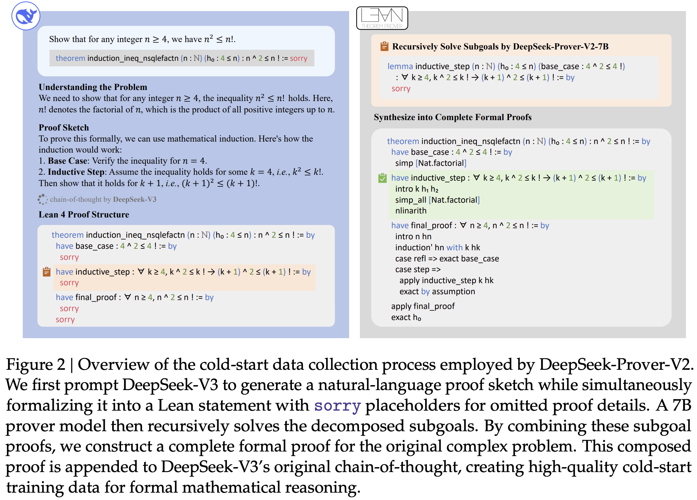
A 7-billion parameter prover model (DSPv2-7B) attempts to replace each sorry with valid Lean tactics. A strict filter selects data: only if the 7B model successfully proves every single subgoal, resulting in a complete Lean proof verified by the compiler, is the instance kept. For these successful instances, the original natural language plan is paired with the complete, verified Lean 4 proof ({NL Plan, Verified Lean Proof}) to form the cold-start dataset.
Subgoals from these successful decompositions also generate curriculum learning tasks (Figure 3) used in model training. These tasks involve proving subgoals directly or with preceding subgoals provided as premises. Providing premises aims to train contextual reasoning, mirroring lemma usage in proofs, though the paper does not present evidence isolating the benefit of this structure compared to proving subgoals independently.
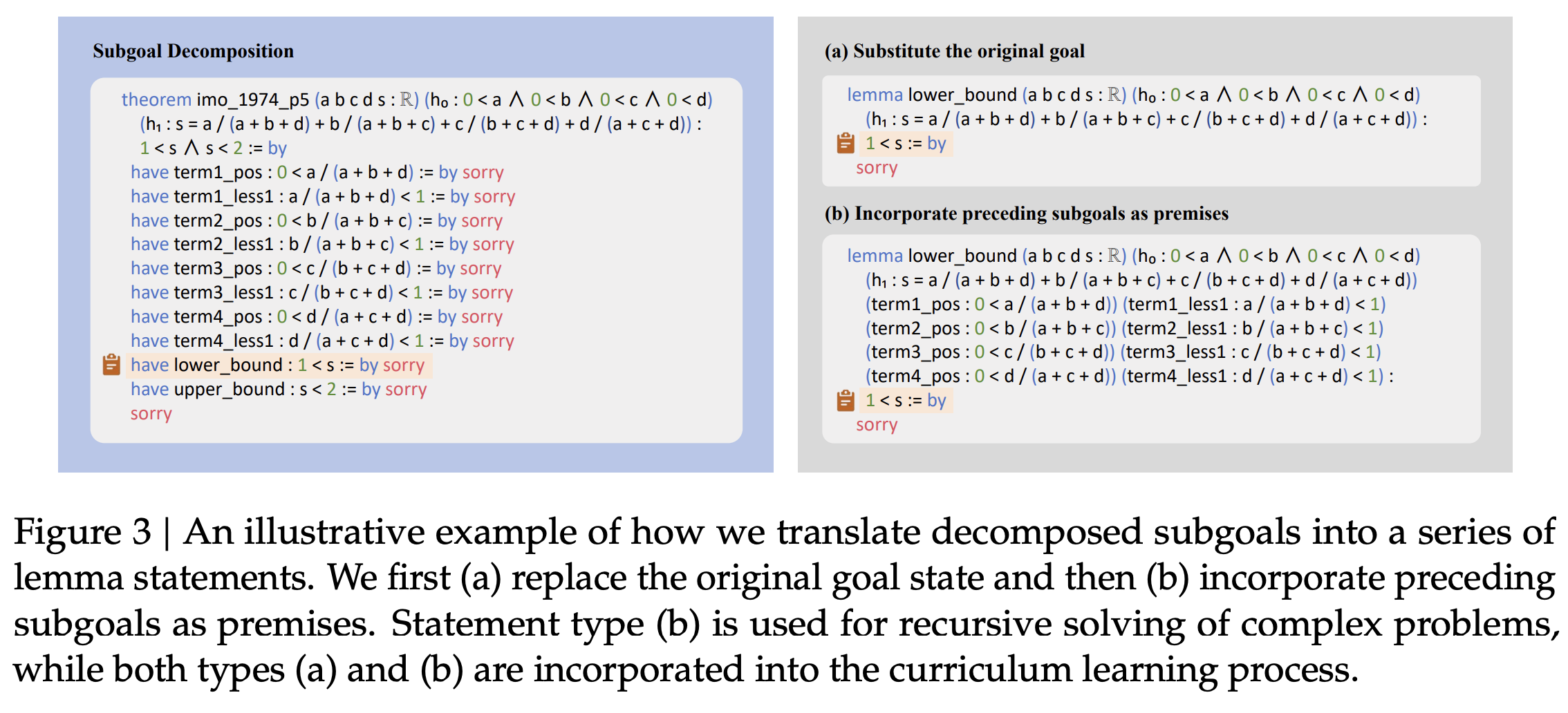
Reinforcement Learning:
Models, initialized via supervised fine-tuning, are trained using Group Relative Policy Optimization (GRPO). GRPO is a policy gradient method (see Basic facts about policy gradients for an intro to policy gradients) updating policies based on relative proof success rankings within a sampled batch, differing from methods using explicit value functions. The primary reward is binary (+1 for verified proof). An auxiliary structural consistency reward encourages alignment with the DeepSeek-V3 plan early in training by “enforcing the inclusion of all decomposed have-structured lemmas in the final proof.”
Generation Modes: Distinct prompts (Appendix A) elicit two modes: non-CoT (concise Lean code) for efficiency, and CoT (code with NL comments) for interpretability/accuracy. The non-CoT prompt requests code completion directly, while the CoT prompt first asks for a proof plan before generating the commented code.
Evaluation
The DeepSeek-Prover-V2 models were evaluated on Lean 4 formalizations using several benchmarks. Test sets were reserved for evaluation only.
Established benchmarks included MiniF2F, ProofNet, and PutnamBench. MiniF2F contains 488 elementary math problems from competitions (AIME, AMC, IMO) and the MATH dataset, previously formalized; the paper uses the standard valid/test splits, incorporating miniF2F-valid into training curriculum. ProofNet offers 371 undergraduate pure math problems (analysis, algebra, topology) translated from Lean 3 formalizations; the evaluation uses the ProofNet-test split. PutnamBench uses problems from the Putnam Mathematical Competition (1962-2023) covering diverse undergraduate topics, formalized in Lean 4; the evaluation used 649 problems compatible with Lean 4.9.0.
The authors also introduced ProverBench, a new 325-problem benchmark formalized for this work. It aims to span high-school competition and undergraduate levels. It includes 15 recent AIME problems (2024-25) focused on number theory and algebra (Table 7 details selection), filtering out geometry and combinatorics. The remaining 310 problems come from textbooks and tutorials covering number theory, algebra (elementary, linear, abstract), calculus, analysis (real, complex, functional), and probability (Table 8 shows distribution). ProverBench is available via the paper’s GitHub repository.
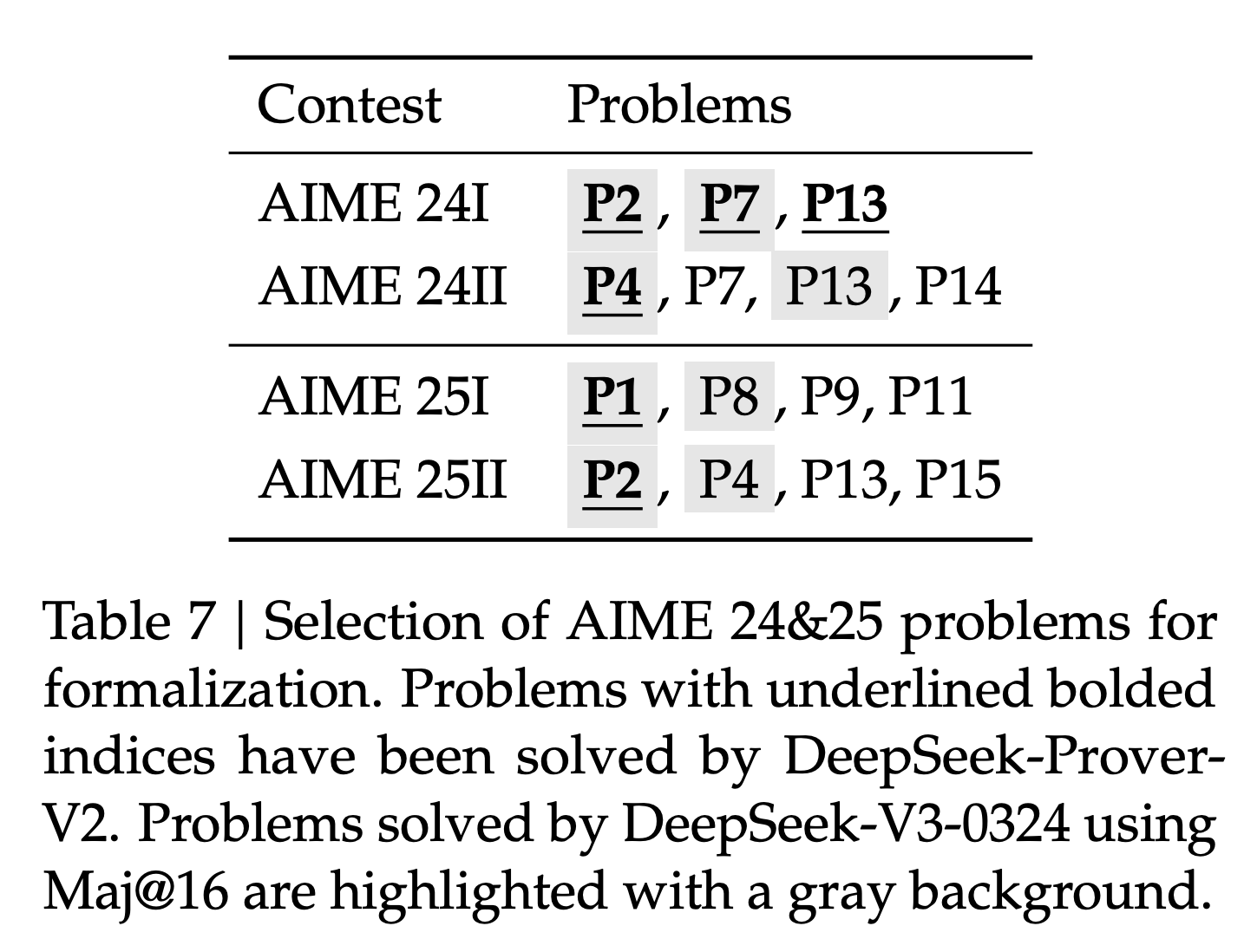
. |
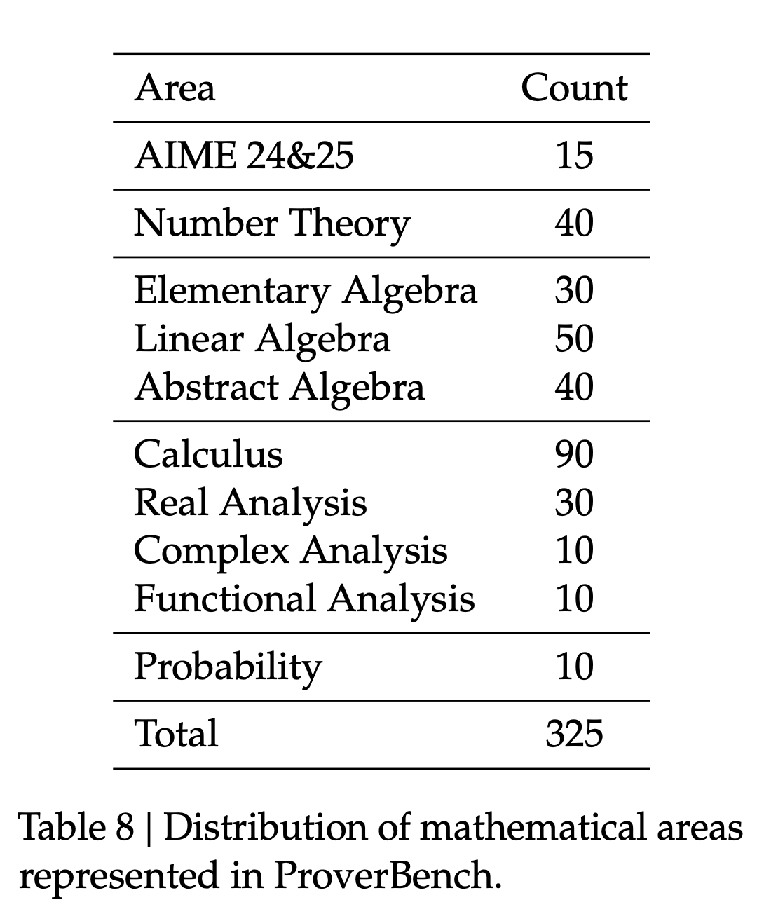
|
Results
-
Performance: On MiniF2F-test (Olympiad math), DSPv2-671B (CoT) achieved 88.9% Pass@8192 and 82.4% Pass@32, exceeding prior state-of-the-art (Table 1). On PutnamBench (competition math), it solved 49/658 problems (Pass@1024, Table 4). Figure 1 shows benchmark graphs.
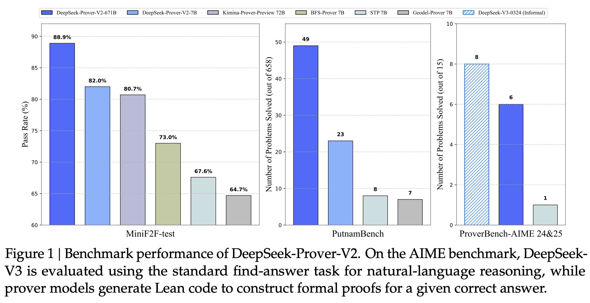
-
ProverBench: On the AIME subset of the authors’ new benchmark, DSPv2-671B (CoT, formal proof) solved 6/15 problems, versus 8/15 solved by DeepSeek-V3 via informal reasoning. (Table 6).
-
Skill Discovery: DSPv2-7B (non-CoT) solved 13 PutnamBench problems missed by the 671B model. It used specific Lean tactics (
Cardinal.toNat,Cardinal.natCast_inj). These tactics are needed because Lean strictly distinguishes types.Cardinalrepresents set size abstractly, whileNatrepresents natural numbers. Even for finite sets, proving properties that rely onNatarithmetic (like specific inequalities) might require explicitly converting aCardinalsize to aNatusingCardinal.toNator using lemmas likeCardinal.natCast_injto relate equalities across types. Standard arithmetic tactics may not automatically bridge this type gap. The 7B model’s RL process apparently favored strategies requiring these tactics for certain problems. (Appendix B examples).
Getting the hang of policy gradients by reframing optimization as RL
We can gain insight into Reinforcement Learning (RL) training mechanisms by taking a general optimization problem and reframing it as a “stateless RL problem.” In this reframing, the task is to find optimal parameters for a probability distribution that generates candidate solutions. The distribution’s parameters are adjusted based on rewards received for sampled solutions, aiming to increase the probability of generating high-reward solutions. This perspective isolates aspects of policy optimization from complexities such as state-dependent decision making.
Note: while writing this I remembered that Mr. Ben Recht wrote a blog post that considered a similar reframing back in 2018.
From Optimization to a Stateless RL
Consider the general problem of finding a vector $w$ that minimizes a loss function $L(w)$:
\[\min_w L(w)\]$L(w)$ can be a deterministic function of $w$. Alternatively, $L(w)$ might represent an expected loss,
\[L(w) = E_{z \sim D_z}[\ell(w,z)]\]where $\ell(w,z)$ is a loss computed for a specific data sample $z$ drawn from a distribution $D_z$.
To transform this into an RL problem, we shift from directly seeking an optimal $w$ to optimizing the parameters $\theta$ of a policy $\pi_\theta(w)$. The policy $\pi_\theta(w)$ is a probability distribution that generates candidate solutions $w$. The RL objective is then to find parameters $\theta$ that maximize the expected reward $J(\theta)$ obtained from these solutions:
\[J(\theta) = E_{w \sim \pi_\theta(w)}[R(w)]\]If the policy is $\pi_\theta(w) = N(w|\mu, \sigma^2)$ and the reward is $R(w) = -L(w)$, with $L(w)$ uniquely minimized at $w^* $, then $J(\theta)$ is maximized as the policy mean $\mu$ approaches $w^*$ and the standard deviation $\sigma$ approaches $0^+$. In this limit, the policy effectively concentrates its mass at $w^* $.
In this construction:
- The policy $\pi_\theta(w)$, parameterized by $\theta$, is the distribution used to sample candidate solutions $w$.
- An action corresponds to sampling a solution $w$ from $\pi_\theta(w)$.
- The environment is effectively stateless because the reward $R(w)$ for a sampled solution $w$ depends only on $w$.
The definition of the reward $R(w)$ is derived from the original optimization problem. If the goal is to minimize $L(w)$, one reward definition is $R(w) = -L(w)$. If the loss is stochastic, $\ell(w,z)$, then the reward can also be stochastic, for example, $R(w,z) = -\ell(w,z)$. In this stochastic reward case, the objective becomes $J(\theta) = E_{w \sim \pi_\theta(w)}[E_{z \sim D_z}[R(w,z)]]$.
Example Reward Formulations
The way $R(w)$ (or $R(w,z)$) is defined based on $L(w)$ or $\ell(w,z)$ directly influences the information available to the learning algorithm. To explore these effects, we consider several reward structures:
- True Reward: $R(w) = -L(w)$.
- This reward provides direct information about $L(w)$ for each sampled $w$.
- Unbiased Randomized Reward: $R(w,z) = -\ell(w,z)$, where $z \sim D_z$.
- This reward uses individual data instances $z$. $R(w,z)$ is noisy, but $\mathbb{E}_z[R(w,z)] = -L(w)$.
- Proxy Rewards (via a fixed batch): $R(w) = -\frac{1}{|S_{train}|} \sum_{z_i \in S_{train}} \ell(w,z_i)$. $S_{train}$ is a fixed data batch.
- If $S_{train}$ is unrepresentative, optimizing this $R(w)$ illustrates RL with a learned proxy reward.
- Sparse Rewards: $R(w) = \mathbb{1}_{-L(w) > \text{tol}}$, where $\text{tol}$ is a threshold.
- This yields a binary signal. If the condition is met infrequently, the reward is sparse.
The Policy Gradient in a Stateless Setting
The Policy Gradient Theorem (PGT) provides a method for computing $\nabla_\theta J(\theta)$. (A PGT derivation is in a previous post). For the stateless problem, the policy gradient is:
\[\nabla_\theta J(\theta) = \mathbb{E}_{w \sim \pi_\theta(w), z \sim D_z}[ \nabla_\theta \log \pi_\theta(w) R(w,z) ] \quad (*)\](If $R(w)$ is deterministic, omit expectation over $z$). A stochastic estimate of $\nabla_\theta J(\theta)$ is $\hat{g}_t = \nabla_\theta \log \pi_\theta(w_t) R(w_t, z_t)$, using samples $w_t \sim \pi_{\theta_t}(w)$ and $z_t \sim D_z$. Policy parameters can then be updated via stochastic gradient ascent:
\[\theta \leftarrow \theta + \alpha \hat{g}_t\]Properties of the Policy Gradient Estimator
The estimator $\hat{g}_t = \nabla_\theta \log \pi_\theta(w_t) R(w_t, z_t)$ is an unbiased estimate of $\nabla_\theta J(\theta)$. The variance of this estimator, $\text{Var}(\hat{g}_t) = \mathbb{E}[(\nabla_\theta \log \pi_\theta(w) R(w,z))^2] - (\nabla_\theta J(\theta))^2$, can be large. This variance impacts learning stability and speed.
For example, consider a policy $\pi_\theta(w) = N(w | \mu, \sigma^2 I_d)$ for $w \in \mathbb{R}^d$. Let parameters be $\theta = (\mu, \psi)$, where $\psi = \log\sigma$ ensures $\sigma = e^\psi > 0$. The score function for $\mu$ is
\[\nabla_\mu \log \pi_\theta(w) = (w-\mu)/\sigma^2.\]The variance of the $\mu$-component of $\hat{g}_t$, $\hat{g}_{\mu,t}$, involves $E[|(w-\mu)/\sigma^2|^2 R(w,z)^2]$. The term $E[|w-\mu|^2/\sigma^4]$ contributes a factor scaling as $d/\sigma^2$. Thus, $\text{Var}(\hat{g}_{\mu,t})$ can scale proportionally to $d/\sigma^2$ multiplied by terms related to $R(w,z)$. This $1/\sigma^2$ dependence shows that as $\sigma \to 0$ (exploitation), $\text{Var}(\hat{g}_{\mu,t})$ can increase if $R(w,z)$ does not also diminish appropriately as $w \to \mu$.
The score for $\psi=\log\sigma$ is
\[\nabla_{\psi} \log \pi_\theta(w) = (\|w-\mu\|^2/\sigma^2 - d),\]where $d$ is the dimension of $w$. The variance of its gradient estimate also depends on $R(w,z)$ and $\sigma$.
Note that an interesting consequence of optimization $L$ via the PGT approach is that $R(w,z)$ can be non-differentiable with respect to $w$. Indeed, we only need to calculate the gradient for policy parameters. This flexibility is exchanged for managing the variance of $\hat{g}_t$. Well, that and the fact that $J$ is generally nonconvex in $\sigma$, even if $L$ is convex.
Aside: Connection to Gaussian Smoothing
If the policy is $w \sim N(\mu, \sigma_0^2 I_d)$ with fixed $\sigma_0^2$ (so $\theta = \mu$), and $R(w) = -L(w)$, then
\[J(\mu) = E_{w \sim N(\mu, \sigma_0^2 I_d)}[-L(w)] = -L_{\sigma_0}(\mu),\]where
\[L_{\sigma_0}(\mu) = E_{w \sim N(\mu, \sigma_0^2 I_d)}[L(w)]\]is the Gaussian-smoothing of the function $L(\cdot)$ evaluated at $\mu$. The policy gradient $\nabla_\mu J(\mu)$ is then $-\nabla_\mu L_{\sigma_0}(\mu)$. Thus, PGT here performs stochastic gradient descent on a smoothed version of $L$. This links PGT to zeroth-order optimization methods.
Variance of the gradient, stepsize selection, and gradient clipping
Recall that we wish to maximize $J(\theta)$ via the stochastic gradient ascent update $\theta \leftarrow \theta + \alpha \hat{g}_t$. Two primary considerations for SGA are the variance of $\hat{g}_t$ and the selection of stepsize $\alpha$.
Variance Reduction
Baselines: In the stateless setting,
\[V^{\pi_\theta} = E_{w \sim \pi_\theta(w)}[R(w)]\]is the expected reward under the policy. The advantage is
\[A^{\pi_\theta}(w') = R(w') - V^{\pi_\theta}.\]Subtracting a baseline $b_t \approx V^{\pi_\theta}$ from the reward:
\[\hat{g}_t = \nabla_\theta \log \pi_\theta(w_t) (R(w_t, z_t) - b_t)\]One way to estimate $V^{\pi_\theta}$ online is using an exponential moving average of rewards. This provides $b_t$. The centered term $(R(w_t,z_t) - b_t)$ can yield a lower variance $\hat{g}_t$.
Batch Gradient Estimator: One can average $\hat{g}_t$ over a mini-batch of $N_s$ independent samples $w_j \sim \pi_\theta(w)$ (each with its own $R(w_j)$ or $R(w_j, z_j)$). This forms $\bar{g}_t = \frac{1}{N_s} \sum_{j=1}^{N_s} \hat{g}_{t,j}$. In this case,
\[\text{Var}(\bar{g}_t) = \text{Var}(\text{single sample } \hat{g}_t)/N_s.\]This reduces variance at the cost of $N_s$ reward evaluations per policy update.
Stepsize Selection and Convergence
The objective $J(\theta)$ is generally non-convex. For non-convex $J(\theta)$, convergence rate analysis focuses on metrics like $E[|\nabla J(\theta_k)|^2] \to 0$ (or to a noise floor for constant $\alpha$). In more restricted settings, for example, if $J(\theta)$ is (locally) strongly convex around an optimum $\theta^*$, metrics like $E[|\theta_k-\theta^*|^2]$ or $J(\theta^*) - J(\theta_k)$ can be analyzed. The stepsize (or learning rate1) $\alpha$ affects convergence. (if none of this is familiar to you, see my lecture notes on stochastic gradient descent for mean estimation)
-
Constant Stepsize: For a constant $\alpha$, $\theta_k$ oscillates around a region where $\nabla J(\theta) \approx 0$. A convergence metric $M_k(\alpha)$ (e.g., $E[|\nabla J(\theta_k)|^2]$ for non-convex or $E[|\theta_k-\theta^*|^2]$ for locally convex) usually scales as:
\[M_k(\alpha) \approx \frac{C_0 \cdot (\text{Initial Error})}{h(k) \cdot \alpha} + \frac{C_1 \cdot \alpha \cdot \text{Var}(\text{single sample } \hat{g}_t)}{N_s}\]where $h$ is some function of $k$ (e.g., $k^{-1/2}$) and $N_s$ is the batch size for $\hat{g}_t$ ($N_s=1$ if no batching). As $k \to \infty$, the first term (bias reduction) vanishes, leaving the second term (noise floor). A larger $\alpha$ speeds initial progress but gives a higher noise floor.
-
Diminishing Stepsize: For $M_k(\alpha_k) \to 0$, $\alpha_k$ must diminish, for instance, satisfying the Robbins-Monro conditions: $\sum_{k=0}^\infty \alpha_k = \infty$ and $\sum_{k=0}^\infty \alpha_k^2 < \infty$.
There are of course issues with these bounds when we take $\sigma$ to zero, since the variance explodes. To actually achieve convergence, we would need to increase the batch size sufficiently fast. Or, we could
Clip the gradients
Gradient clipping replaces $\hat{g}_t$ with $c\frac{\hat{g}_t}{||\hat{g}_t||}$ if $||\hat{g}_t|| > c$ for a user specified constant $c$. Since the gradient of the score function explodes as $\sigma$ tends to zero, this becomes necessary.
Illustrative experiments: Policy Gradient for a Quadratic Loss
We apply these concepts to an agent (everything’s an agent now!) learning to sample $w$ to minimize
\[L(w) = \frac{1}{2}(w - w^\ast)^2\]for a target $w^\ast$.
A stochastic version of the loss is
\[\ell(w,z) = \frac{1}{2}(w -(w^\ast + z))^2,\]where $z \sim N(0, \sigma_z^2)$.
The agent’s policy $\pi_\theta(w)$ is $N(w|\mu, \sigma^2)$, for scalar $w$ (i.e., $d=1$). The learnable parameters are $\theta = (\mu, \psi)$, where $\psi = \log\sigma$. This parameterization ensures $\sigma = e^\psi > 0$ when $\psi$ is optimized without constraints.
We now present results from numerical experiments applying the policy gradient approach to the quadratic loss $L(w) = \frac{1}{2}(w - w^\ast)^2$ with target $w^\ast=5.0$. All experiments start from an initial policy $N(0,4)$ and use gradient clipping with norm 10.0. We examine the five reward formulations (R1-R4). For R1 and R2, we investigate the effects of learning rate, baselines, diminishing stepsizes, and batching. For R3, R4, and R5, we show specific illustrative runs.
R1: True Reward
The reward is $R(w) = -L(w) = -\frac{1}{2}(w - w^\ast)^2$. Runs use $10^4$ episodes.
Learning Rate Comparison (Set A):
 Figure 1: R1 (True Reward) - Learning Rate Comparison. Compares constant $\alpha \in {0.01, 0.001, 0.0001}$. All use EMA baseline, $N_s=1$. Higher $\alpha$ converges $\mu$ faster towards $w^\ast=5.0$ and decreases $\sigma$ faster. Lower $\alpha$ converges slower.
Baseline Comparison (Set B):
 Figure 2: R1 (True Reward) - Baseline Comparison. Compares EMA baseline vs. no baseline ($b_t=0$) for $\alpha=0.001$, $N_s=1$. The EMA baseline stabilizes the decrease of $\sigma$, avoiding the large initial increase seen without a baseline.
Stepsize Schedule Comparison (Set C):
 Figure 3: R1 (True Reward) - Stepsize Schedule Comparison. Compares constant $\alpha=0.01$ vs. a diminishing schedule starting at $\alpha_0=0.01$. Both use EMA baseline, $N_s=1$. Performance is comparable over this number of episodes; the diminishing schedule shows slightly less oscillation in $\mu$ near the end.
Batch Gradient Estimator Comparison (Set D):
 Figure 4: R1 (True Reward) - Batch Gradient Comparison. Compares $N_s=1$ vs. $N_s=10$. Both use $\alpha=0.001$, EMA baseline. Using $N_s=10$ results in visibly smoother trajectories for $\mu$ and $\sigma$, demonstrating variance reduction per update.
R2: Randomized Reward
The reward is $R(w,z) = -\ell(w,z) = -(\frac{1}{2}(w - (w^\ast+z))^2)$, where $z \sim N(0, 1)$. Runs use $10^4$ episodes.
Learning Rate Comparison (Set A):
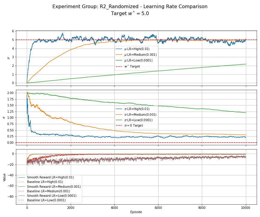 Figure 5: R2 (Randomized Reward) - Learning Rate Comparison. Compares constant $\alpha \in {0.01, 0.001, 0.0001}$. All use EMA baseline, $N_s=1$. Higher $\alpha$ converges faster but exhibits significant oscillations around $w^\ast=5.0$ (noise floor). Lower $\alpha$ reduces oscillation variance but converges slower.
Baseline Comparison (Set B):
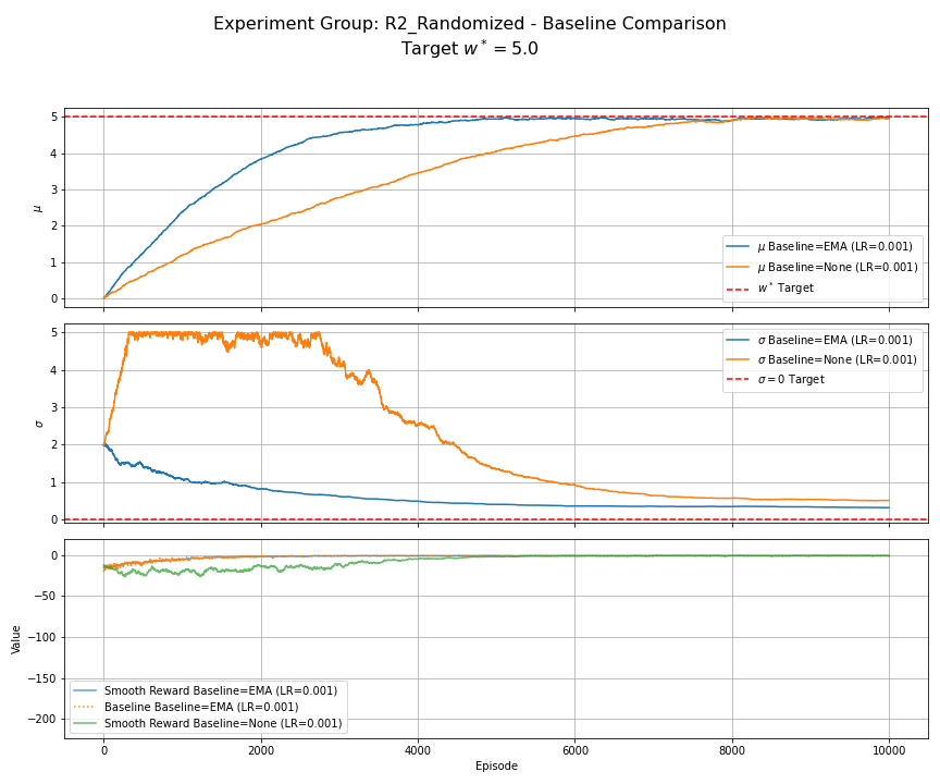 Figure 6: R2 (Randomized Reward) - Baseline Comparison. Compares EMA baseline vs. no baseline ($b_t=0$) for $\alpha=0.001$, $N_s=1$. The EMA baseline enables stable convergence of $\mu$ and $\sigma$. Without the baseline, learning is highly unstable, especially for $\sigma$.
Stepsize Schedule Comparison (Set C):
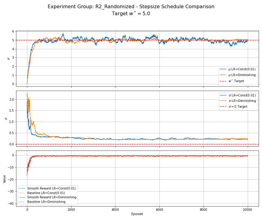 Figure 7: R2 (Randomized Reward) - Stepsize Schedule Comparison. Compares constant $\alpha=0.01$ vs. diminishing schedule starting at $\alpha_0=0.01$. Both use EMA baseline, $N_s=1$. The diminishing stepsize significantly reduces the oscillations (noise floor) seen with the constant stepsize.
Batch Gradient Estimator Comparison (Set D):
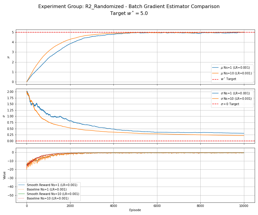 Figure 8: R2 (Randomized Reward) - Batch Gradient Comparison. Compares $N_s=1$ vs. $N_s=10$. Both use $\alpha=0.001$, EMA baseline. Using $N_s=10$ yields noticeably smoother trajectories for $\mu$ and $\sigma$, reducing the impact of reward noise.
R3: Proxy Reward Optimization (Fixed Batch)
This experiment investigates optimizing a proxy reward based on a fixed batch $S_{train}$. The reward is $R(w) = -\text{avg}_{z_i \in S_{train}}[\ell(w, z_i)]$, where $\ell(w, z_i) = \frac{1}{2}(w - (w^\ast + z_i))^2$ and $S_{train}$ contains $N_s$ samples of $z_i \sim N(0,1)$ generated once. We compare results for batch sizes $N_s=1, 5, 10, 20$. All runs use $\alpha=0.01$, EMA baseline, and $10^4$ episodes.
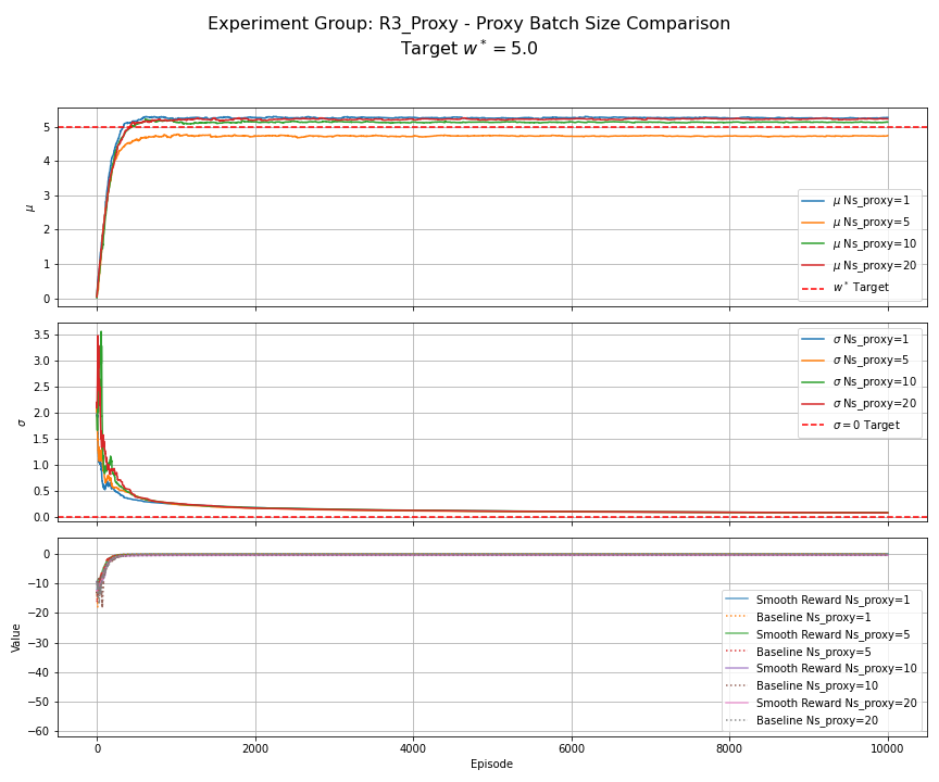 Figure 9: R3 Proxy Reward (Fixed Batch) - Batch Size Comparison. Compares optimizing the empirical average reward over fixed batches $S_{train}$ of size $N_s \in {1, 5, 10, 20}$. All use $\alpha=0.01$, EMA baseline. Convergence of $\mu$ appears closer to the true $w^\ast=5.0$ as $N_s$ increases, illustrating how optimizing a small fixed batch (a proxy objective) can lead to solutions biased away from the true optimum.
R4: Discrete Sparse Reward
The reward is $R(w) = 1$ if $(w-w^\ast)^2 < 0.25$, else $0$. We show a single run with $\alpha=0.01$, EMA baseline, $N_s=1$, for $5 \times 10^4$ episodes.
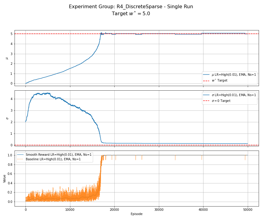 Figure 10: R4 (Discrete Sparse Reward) - Single Run. Reward is 1 if $|w-w^\ast|<0.5$, else 0. Uses $\alpha=0.01$, EMA baseline, $N_s=1$. Learning shows a long initial phase with slow progress in $\mu$ while $\sigma$ increases (exploration). Once the rewarding region is found, $\mu$ converges towards $w^\ast$ and $\sigma$ decreases.
Footnotes
-
I think I’ve completely given up and no longer care whether I say stepsize or learning rate. ↩
All roads lead to likelihood: the value of reinforcement learning in fine-tuning
The paper “All Roads Lead to Likelihood: The Value of Reinforcement Learning in Fine-Tuning” examines why online, two-stage fine-tuning procedures like RLHF often appear to outperform direct offline methods such as DPO in aligning language models with human preferences. The core of the paper establishes an algebraic equivalence between these approaches under specific assumptions about the reward model’s structure, and then hypothesizes that observed empirical differences arise from a “generation-verification gap,” where learning a simpler reward model (verifier) separately is easier than jointly learning a policy (generator) and its implicit reward.
The foundation for modeling preferences is the Bradley-Terry (BT) model, where the probability of preferring trajectory $\xi_1$ over $\xi_2$ is
\[P(\xi_1 \succ \xi_2 | r) = \sigma(r(\xi_1) - r(\xi_2)),\]with $r(\xi)$ being a scalar reward for trajectory $\xi$ and $\sigma$ the sigmoid function. Offline Direct Preference Optimization (DPO) directly optimizes a policy $\pi \in \Pi$ (where $\Pi$ is the class of policies) by defining an implicit “local” reward
\[r_\pi(\xi) = \sum_{h=0}^{H-1} \log \pi(a_h|s_h).\]The DPO objective is then to find the policy $\hat{\pi}_{DPO}$ that maximizes the log-likelihood of observed preferences:
\[\hat{\pi}_{DPO} = \underset{\pi \in \Pi}{\text{argmax}} \sum_{(\xi^+, \xi^-) \in D} \log \sigma(r_\pi(\xi^+) - r_\pi(\xi^-)).\]In contrast, online RLHF first learns an explicit “global” reward model $\hat{r}_G$ from a class of reward functions $R$ by maximizing:
\[\hat{r}_G = \underset{r_G \in R}{\text{argmax}} \sum_{(\xi^+, \xi^-) \in D} \log \sigma(r_G(\xi^+) - r_G(\xi^-)).\]Subsequently, it learns a policy $\hat{\pi}_{RLHF}^*$ using this $\hat{r}_G$. The objective for this policy optimization involves maximizing a combination of expected reward and the policy’s entropy. The causal entropy of a policy $\pi$, denoted $H(\pi)$, is defined as the expected sum of the negative log probabilities of actions taken under that policy, over the course of a trajectory $\xi = (s_0, a_0, \dots, s_{H-1}, a_{H-1}, s_H)$ generated by $\pi$:
\[H(\pi) = \mathbb{E}_{\xi \sim \pi} \left[ -\sum_{h=0}^{H-1} \log \pi(a_h|s_h) \right].\]Here, the expectation $\mathbb{E}_{\xi \sim \pi}$ is over trajectories where $s_0$ is drawn from an initial state distribution and subsequent actions $a_h$ are drawn from $\pi(\cdot|s_h)$. The policy optimization objective, as ‘per the principle of maximum entropy RL’, is:
\[\hat{\pi}_{RLHF}^* = \underset{\pi' \in \Pi}{\text{argmax}} \left( \mathbb{E}_{\xi \sim \pi'} [\hat{r}_G(\xi)] + H(\pi') \right).\]One can show that the policy yields a trajectory distribution $P_{\hat{\pi}_{RLHF}^* }^* (\xi) \propto \exp(\hat{r}_G(\xi))$.
The paper’s first main result (Theorem 2.2) demonstrates an algebraic equivalence: if the global reward model class $R$ in RLHF is constrained to be $R(\Pi)$ (i.e., rewards must have the form $r_{\pi’}(\xi) = \sum_h \log \pi’(a_h|s_h)$ for some policy $\pi’ \in \Pi$), then the two approaches are identical. Under this constraint, Stage 1 of RLHF becomes:
\[\hat{r}_G = \underset{r_{\pi'} \in R(\Pi)}{\text{argmax}} \sum_{(\xi^+, \xi^-) \in D} \log \sigma(r_{\pi'}(\xi^+) - r_{\pi'}(\xi^-)).\]The policy $\pi’$ parameterizing the optimal $r_{\pi’}$ in this expression is, by definition, $\hat{\pi}_{DPO}$. Thus, the learned reward model is $\hat{r}_G = r_{\hat{\pi}_{DPO}}(\xi)$.
Stage 2 of RLHF then seeks a policy $\pi^*$ such that its trajectory distribution satisfies $P_{\pi^* }^* (\xi) \propto \exp(r_{\hat{\pi}_{DPO}}(\xi))$. Substituting $r_{\hat{\pi}_{DPO}}(\xi) = \sum_h \log \hat{\pi}_{DPO}(a_h|s_h)$, we get:
\[P_{\pi^*}^*(\xi) \propto \exp\left(\sum_h \log \hat{\pi}_{DPO}(a_h|s_h)\right) = \prod_h \hat{\pi}_{DPO}(a_h|s_h).\]This implies the optimal policy $\pi^*$ from RLHF Stage 2 is $\hat{\pi}_{DPO}$. Thus, when the reward model architecture is restricted in this specific way, RLHF simply rearranges the DPO optimization.
To explain the empirically observed advantage of online methods, the paper proposes the “generation-verification gap” hypothesis (H6). This posits that the true underlying reward structure $r^* $ dictating preferences might be “simple” (belonging to a class $R_{sim}$ that is easy to learn) and that an unconstrained global reward model in RLHF’s Stage 1 can effectively learn this $r^* $. If DPO’s implicit reward $r_\pi(\xi)$ struggles to represent this $r^* $ with a policy $\pi$ that is also easy to find, or if the joint optimization of finding such a $\pi$ is inherently harder, then RLHF gains an advantage. RLHF decouples the problem: first learn $r^* \in R_{sim}$, then derive a policy for it. DPO attempts to find a policy $\pi$ whose structure $r_\pi$ simultaneously captures $r^*$ and defines an optimal policy. A related result (Theorem 3.1) formalizes that if DPO’s search were restricted to policies optimal for some $r \in R_{sim}$, it would match RLHF’s outcome.
The paper presents experiments where manipulating task or reward complexity (e.g., very short trajectories, or using a complex predefined reward like ROUGE-L) alters the performance gap between online and offline methods. These are interpreted as supporting H6 by showing that when the generation-verification gap is presumed to be small (verification is as hard as generation, or generation is trivially easy), the online advantage diminishes.
Basic facts about policy gradients
Problem setup
The goal of Reinforcement Learning (RL) is for an agent to learn “optimal” behavior through interaction with an environment. The agent’s decisions are guided by a policy $\pi_\theta(a|s)$, parameterized by $\theta$. The objective is to find $\theta$ that maximizes
\[J(\theta) = E_{\tau \sim \pi_\theta}[G_0],\]Here, $G_0 = \sum_{k=0}^\infty \gamma^k r_{k+1}$ is the total discounted return for a trajectory $\tau=(s_0, a_0, r_1, s_1, \dots)$ generated by following policy $\pi_\theta$ from an initial state $s_0$ drawn from a distribution $p_0(s_0)$ with $\gamma \in [0,1]$ being the “discount factor.” The distribution $p_0(s_0)$ specifies the probability of starting an episode in state $s_0$.
Value functions and Bellman equations
To evaluate policies, we define value functions. These functions rely on the concept of the return from a generic time step $t$, $G_t = \sum_{k=0}^\infty \gamma^k r_{t+k+1}$. Importantly, in this definition of $G_t$, the discount $\gamma^k$ applies to the $k$-th reward after $r_t$, meaning the “discount clock” effectively resets at time $t$.
- The State-Value Function $V^\pi(s) = E_\pi[G_t | s_t=s]$ is the expected return from starting in state $s$ and following policy $\pi$.
- The Action-Value Function $Q^\pi(s,a) = E_\pi[G_t | s_t=s, a_t=a]$ is the expected return from starting in state $s$, taking action $a$, and then following policy $\pi$.
Because the environment and policy are stationary, the specific value of $t$ used in the definition does not change the resulting values $V^\pi(s)$ or $Q^\pi(s,a)$; they are functions of state (and action) only.
These value functions are related by the identity:
\[V^\pi(s) = \sum_a \pi(a|s) Q^\pi(s,a).\]They satisfy the Bellman expectation equations, which express values recursively. Let $P(s’|s,a)$ be the state transition probability and $R(s,a,s’)$ be the expected immediate reward for $(s,a,s’)$.
\[\begin{aligned} V^\pi(s) &= \sum_a \pi(a|s) \sum_{s'} P(s'|s,a) [R(s,a,s') + \gamma V^\pi(s')], \\ Q^\pi(s,a) &= \sum_{s'} P(s'|s,a) [R(s,a,s') + \gamma V^\pi(s')]. \end{aligned}\]These equations state that the value of a state (or state-action pair) under $\pi$ is the sum of the expected immediate reward and the discounted expected value of subsequent states encountered by following $\pi$.
The policy gradient theorem
The Policy Gradient Theorem provides an expression for $\nabla_\theta J(\theta)$. It’s useful because we can compute unbiased estimates of the gradient from samples of trajectories generated by $\pi_\theta$.
Let $P(\tau|\theta)$ be the probability of trajectory $\tau$ under policy $\pi_\theta$.
\[J(\theta) = \sum_\tau P(\tau|\theta) G_0(\tau).\]Then, $\nabla_\theta J(\theta) = \sum_\tau \nabla_\theta P(\tau|\theta) G_0(\tau)$. Using the log-derivative trick,
\[\nabla_\theta P(\tau|\theta) = P(\tau|\theta) \nabla_\theta \log P(\tau|\theta),\]we get:
\[\nabla_\theta J(\theta) = \sum_\tau P(\tau|\theta) (\nabla_\theta \log P(\tau|\theta)) G_0(\tau) = E_{\tau \sim \pi_\theta} [(\nabla_\theta \log P(\tau|\theta)) G_0(\tau)].\]The probability of a trajectory is $P(\tau|\theta) = p_0(s_0) \prod_{t=0}^\infty \pi_\theta(a_t|s_t) P(s_{t+1}|s_t, a_t)$. Thus, $\log P(\tau|\theta) = \log p_0(s_0) + \sum_{t=0}^\infty (\log \pi_\theta(a_t|s_t) + \log P(s_{t+1}|s_t, a_t))$. The gradient $\nabla_\theta$ only affects terms involving $\pi_\theta$:
\[\nabla_\theta \log P(\tau|\theta) = \sum_{t=0}^\infty \nabla_\theta \log \pi_\theta(a_t|s_t).\]Substituting this back, we get:
\[\nabla_\theta J(\theta) = E_{\tau \sim \pi_\theta} \left[ \left( \sum_{t=0}^\infty \nabla_\theta \log \pi_\theta(a_t|s_t) \right) G_0(\tau) \right]\]It can be shown that terms $\nabla_\theta \log \pi_\theta(a_k|s_k)$ for $k < t$ are uncorrelated with rewards $r_{t’}$ for $t’ \ge t$ given $s_k, a_k$. This “causality” argument allows us to replace $G_0(\tau)$ with $G_k(\tau)$ for the term $\nabla_\theta \log \pi_\theta(a_k|s_k)$, leading to a common form:
\[\nabla_\theta J(\theta) = E_{\tau \sim \pi_\theta} \left[ \sum_{t=0}^\infty \nabla_\theta \log \pi_\theta(a_t|s_t) G_t \right] \quad (*)\]In this expression, $G_t = \sum_{k=0}^\infty \gamma^k r_{t+k+1}$ is the full discounted return experienced from state $s_t$ onwards within the trajectory $\tau$. The term $\nabla_\theta \log \pi_\theta(a_t|s_t)$ is often called the “score function” for action $a_t$ in state $s_t$. The product of the score function and $G_t$ determines the direction and magnitude of the update for actions taken along a trajectory.
The gradient $E_{\tau \sim \pi_\theta} \left[ \sum_{t=0}^\infty \nabla_\theta \log \pi_\theta(a_t|s_t) G_t \right]$ is typically estimated using Monte Carlo sampling. For a single trajectory $\tau^{\text{sample}} \sim \pi_\theta$, an unbiased estimate of this gradient is $\sum_{t=0}^\infty (\nabla_\theta \log \pi_\theta(a_t|s_t)) G_t^{\text{sample}}$. A stochastic gradient ascent update then uses this estimate:
\[\theta \leftarrow \theta + \alpha \left( \sum_{t=0}^\infty (\nabla_\theta \log \pi_\theta(a_t|s_t)) G_t^{\text{sample}} \right)\]where $G_t^{\text{sample}}$ is the return from the sampled trajectory $\tau^{\text{sample}}$. In practice, the sum is truncated at a finite horizon $H$.
Connection to value functions
To connect this to value functions, we can utilize the definition of the action-value function, $Q^{\pi_\theta}(s_t,a_t) = E_{\pi_\theta}[G_t | s_t, a_t]$. This states that $Q^{\pi_\theta}(s_t,a_t)$ is the expected value of the random variable $G_t$, conditioned on having been in state $s_t$ and taken action $a_t$, and subsequently following policy $\pi_\theta$.
Using the law of total expectation ($E[X] = E_Y[E[X|Y]]$), we can rewrite the expectation in $(*)$:
\[\begin{aligned} \nabla_\theta J(\theta) &= E_{\tau \sim \pi_\theta} \left[ \sum_{t=0}^\infty \nabla_\theta \log \pi_\theta(a_t|s_t) G_t \right] \\ &= \sum_{t=0}^\infty E_{\tau \sim \pi_\theta} \left[ \nabla_\theta \log \pi_\theta(a_t|s_t) G_t \right] \\ &= \sum_{t=0}^\infty E_{(s_t,a_t) \text{ in } \tau \text{ at step } t} \left[ \nabla_\theta \log \pi_\theta(a_t|s_t) E[G_t | s_t, a_t, \pi_\theta] \right] \\ &= \sum_{t=0}^\infty E_{(s_t,a_t) \text{ in } \tau \text{ at step } t} \left[ \nabla_\theta \log \pi_\theta(a_t|s_t) Q^{\pi_\theta}(s_t,a_t) \right] \end{aligned}\]Here, the expectation $E_{(s_t,a_t) \text{ in } \tau \text{ at step } t}[\cdot]$ denotes averaging over all possible state-action pairs $(s_t, a_t)$ that can occur at time $t$ when trajectories are generated according to $s_0 \sim p_0(s_0)$ and policy $\pi_\theta$. This form, $\nabla_\theta J(\theta) = E_{\tau \sim \pi_\theta} \left[ \sum_{t=0}^\infty \nabla_\theta \log \pi_\theta(a_t|s_t) Q^{\pi_\theta}(s_t,a_t) \right]$, shows that the policy gradient depends on the Q-values of the actions taken.
The Advantage Function: Improving Gradient Estimates
The variance of $G_t$ as an estimator for $Q^{\pi_\theta}(s_t,a_t)$ can be high. We can introduce a state-dependent baseline $b(s_t)$ into the policy gradient expression without changing its expectation:
\[\nabla_\theta J(\theta) = E_{\pi_\theta} [ \sum_t \nabla_\theta \log \pi_\theta(a_t|s_t) (Q^{\pi_\theta}(s_t,a_t) - b(s_t)) ].\]This holds because
\[E_{a_t \sim \pi_\theta(\cdot|s_t)}[\nabla_\theta \log \pi_\theta(a_t|s_t) b(s_t)] = \sum_{a_t} \nabla_\theta \pi_\theta(a_t|s_t) b(s_t) = b(s_t) \nabla_\theta \sum_{a_t} \pi_\theta(a_t|s_t) = 0.\]When using samples $G_t$ in place of $Q^{\pi_\theta}(s_t,a_t)$, the term in the gradient is $\nabla_\theta \log \pi_\theta(a_t|s_t) (G_t - b(s_t))$. The variance of the scalar factor $(G_t - b(s_t))$, conditioned on $s_t$, is minimized by choosing $b(s_t) = E[G_t|s_t] = V^{\pi_\theta}(s_t)$.
Thus, the optimal choice for $b(s_t)$ is $V^{\pi_\theta}(s_t)$. This leads to using the Advantage Function
\[A^{\pi_\theta}(s_t, a_t) = Q^{\pi_\theta}(s_t, a_t) - V^{\pi_\theta}(s_t).\]The policy gradient estimate becomes
\[\sum_t \nabla_\theta \log \pi_\theta(a_t|s_t) (G_t - V_w(s_t)),\]where $V_w(s_t)$ is an estimate of $V^{\pi_\theta}(s_t)$, and $(G_t - V_w(s_t))$ is an estimate of $A^{\pi_\theta}(s_t,a_t)$.
Actor-Critic Methods
Actor-Critic methods learn two distinct components:
- The Actor: A policy $\pi_\theta(a|s)$, parameterized by $\theta$, which determines how the agent behaves.
- The Critic: A state-value function approximator $V_w(s)$, parameterized by $w$, which estimates $V^{\pi_\theta}(s)$, the value of states under the current actor’s policy.
These components are learned concurrently.
Critic Learning: The critic $V_w(s)$ (commonly a neural network) aims to approximate $V^{\pi_\theta}(s)$. It is trained by minimizing a loss function that measures the discrepancy between its predictions and target values derived from experience. For TD(0) learning, after observing a transition $(s_t, a_t, r_{t+1}, s_{t+1})$, the target for $V_w(s_t)$ is
\[y_t = r_{t+1} + \gamma V_w(s_{t+1}).\]The critic’s parameters $w$ are updated to minimize the squared error
\[(y_t - V_w(s_t))^2.\]The gradient of $\frac{1}{2}(y_t - V_w(s_t))^2$ with respect to $w$ is $-(y_t - V_w(s_t))\nabla_w V_w(s_t)$, assuming $y_t$ is treated as a fixed target during differentiation. This is only an approximation of the full gradient step method because the target $y_t$ itself contains $V_w(s_{t+1})$, but its dependency on $w$ is ignored when computing the gradient for the update related to $V_w(s_t)$.
Given this gradient estimate, we can update the critics parameters using the stochastic gradient update:
\[w \leftarrow w + \alpha_w (r_{t+1} + \gamma V_w(s_{t+1}) - V_w(s_t)) \nabla_w V_w(s_t)\]Here, the term
\[\delta_t = r_{t+1} + \gamma V_w(s_{t+1}) - V_w(s_t)\]is called the TD error. This TD error serves as an estimate of the advantage $A^{\pi_\theta}(s_t,a_t)$. To see this relationship, recall $A^{\pi_\theta}(s_t,a_t) = Q^{\pi_\theta}(s_t,a_t) - V^{\pi_\theta}(s_t)$. By definition, $Q^{\pi_\theta}(s_t,a_t) = E_{\pi_\theta}[r_{t+1} + \gamma V^{\pi_\theta}(s_{t+1}) | s_t, a_t]$. So,
\[A^{\pi_\theta}(s_t,a_t) = E_{\pi_\theta}[r_{t+1} + \gamma V^{\pi_\theta}(s_{t+1}) - V^{\pi_\theta}(s_t) | s_t, a_t].\]The TD error $\delta_t = (r_{t+1} + \gamma V_w(s_{t+1})) - V_w(s_t)$ is thus a sample-based estimate of the quantity inside this expectation, where $V_w$ approximates $V^{\pi_\theta}$, and the single observed $(r_{t+1}, s_{t+1})$ pair replaces the expectation over possible next states and rewards.
The TD error $\delta_t$ is a biased estimate of $A^{\pi_\theta}(s_t,a_t)$ if $V_w \neq V^{\pi_\theta}$. However, $\delta_t$ can have lower variance as an advantage estimator compared to the estimate $(G_t^{\text{sample}} - V_w(s_t))$. The return $G_t^{\text{sample}} = r_{t+1} + \gamma r_{t+2} + \gamma^2 r_{t+3} + \dots$ accumulates noise from many future random rewards. The TD error replaces the sum of all future discounted rewards beyond $r_{t+1}$ (i.e., $\gamma G_{t+1}^{\text{sample}}$) with a single bootstrapped estimate $\gamma V_w(s_{t+1})$. If $V_w(s_{t+1})$ is a reasonably stable (even if biased) estimate of $E[G_{t+1}|s_{t+1}]$, then the variance of $r_{t+1} + \gamma V_w(s_{t+1})$ can be much lower than the variance of $r_{t+1} + \gamma G_{t+1}^{\text{sample}}$.
Actor Update: The actor’s parameters $\theta$ are updated using the TD error $\delta_t$ as the estimate of the advantage.
In an online (per-step) setting, the actor update is performed after each transition, using the $\delta_t$ computed for that step:
\[\theta \leftarrow \theta + \alpha_\theta \nabla_\theta \log \pi_\theta(a_t|s_t) \delta_t\]This update adjusts the policy immediately based on the most recent experience.
In a batch setting, after collecting a batch of $N$ transitions and their corresponding TD errors ${(s_i, a_i, \delta_i)}_{i=1}^N$, the actor update sums these contributions:
\[\theta \leftarrow \theta + \alpha_\theta \sum_{i=1}^{N} \nabla_\theta \log \pi_\theta(a_i|s_i) \delta_i\]This update adjusts the policy based on the aggregated experience in the batch. In both cases, the update aims to make actions that lead to a positive TD error (indicating a better-than-expected outcome relative to $V_w(s_t)$) more probable, and actions leading to a negative TD error less probable.
Proximal Policy Optimization (PPO): Constraining Policy Updates for Improved Performance
Policy gradient methods update policy parameters $\theta$. When these updates are based on data collected under a previous policy $\pi_{\theta_{old}}$ (the “old” or behavior policy), and advantage estimates $\hat{A}_t^{\theta_{old}}$ are computed using $\pi_{\theta_{old}}$’s value function, large discrepancies between the new policy $\pi_\theta$ and $\pi_{\theta_{old}}$ can make these advantage estimates inaccurate for evaluating $\pi_\theta$. This can degrade performance. Proximal Policy Optimization (PPO) introduces mechanisms to obtain more reliable policy improvements by constraining how much the policy can change in each update step.
The primary objective is to find a new policy $\pi_\theta$ such that its expected return $J(\theta)$ is greater than $J(\theta_{old})$. A fundamental result from policy iteration theory (related to Kakade & Langford, 2002) provides an exact expression for this performance difference:
\[J(\theta) - J(\theta_{old}) = E_{s \sim d^{\pi_\theta}} \left[ E_{a \sim \pi_\theta(\cdot|s)} [A^{\pi_{\theta_{old}}}(s,a)] \right]\]This identity states that the improvement in expected return is equal to the expected advantage of the actions taken by the new policy $\pi_\theta$, where these advantages $A^{\pi_{\theta_{old}}}(s,a) = Q^{\pi_{\theta_{old}}}(s,a) - V^{\pi_{\theta_{old}}}(s)$ are calculated with respect to the old policy $\pi_{\theta_{old}}$. The outer expectation is over states $s$ visited according to the state visitation distribution $d^{\pi_\theta}$ induced by the new policy $\pi_\theta$.
Directly optimizing $J(\theta) - J(\theta_{old})$ using this expression is challenging because $d^{\pi_\theta}$ depends on the parameters $\theta$ being optimized, making the expectation difficult to compute or differentiate.
To make optimization tractable, we form a local approximation. The first step in this approximation is to replace the expectation over states visited by the new policy, $s \sim d^{\pi_\theta}$, with an expectation over states visited by the old policy, $s \sim d^{\pi_{\theta_{old}}}$. This substitution yields an approximation that is more accurate when $\pi_\theta$ is close to $\pi_{\theta_{old}}$ (implying $d^{\pi_\theta} \approx d^{\pi_{\theta_{old}}}$)
So, we approximate:
\[E_{s \sim d^{\pi_\theta}} \left[ E_{a \sim \pi_\theta(\cdot|s)} [A^{\pi_{\theta_{old}}}(s,a)] \right] \approx E_{s \sim d^{\pi_{\theta_{old}}}} \left[ E_{a \sim \pi_\theta(\cdot|s)} [A^{\pi_{\theta_{old}}}(s,a)] \right]\]Now, the inner expectation $E_{a \sim \pi_\theta(\cdot|s)} [A^{\pi_{\theta_{old}}}(s,a)]$ is still with respect to actions from the new policy $\pi_\theta$. Since we are working with data (trajectories) generated by $\pi_{\theta_{old}}$, we use importance sampling to rewrite this inner expectation in terms of actions $a \sim \pi_{\theta_{old}}(\cdot|s)$:
\[\begin{aligned} E_{a \sim \pi_\theta(\cdot|s)} [A^{\pi_{\theta_{old}}}(s,a)] &= \sum_a \pi_\theta(a|s) A^{\pi_{\theta_{old}}}(s,a) \\ &= \sum_a \pi_{\theta_{old}}(a|s) \frac{\pi_\theta(a|s)}{\pi_{\theta_{old}}(a|s)} A^{\pi_{\theta_{old}}}(s,a) \end{aligned}\]Substituting this back into the approximation for $J(\theta) - J(\theta_{old})$, we obtain a surrogate objective for the performance improvement (ignoring the constant $J(\theta_{old})$ for maximization purposes):
\[L_{\theta_{old}}^{IS}(\theta) = E_{s \sim d^{\pi_{\theta_{old}}}, a \sim \pi_{\theta_{old}}(\cdot|s)} \left[\frac{\pi_\theta(a|s)}{\pi_{\theta_{old}}(a|s)} A^{\pi_{\theta_{old}}}(s,a)\right]\]Here, $\rho_t(\theta) = \frac{\pi_\theta(a_t|s_t)}{\pi_{\theta_{old}}(a_t|s_t)}$ is the importance sampling ratio for a state-action pair $(s_t, a_t)$ from data collected under $\pi_{\theta_{old}}$. This ratio re-weights the advantage $A^{\pi_{\theta_{old}}}(s_t,a_t)$ to account for the relative probability of taking action $a_t$ under $\pi_\theta$ versus $\pi_{\theta_{old}}$. The objective $L_{\theta_{old}}^{IS}(\theta)$ provides an estimate of policy performance improvement, which is a first-order approximation accurate when $\pi_\theta$ is close to $\pi_{\theta_{old}}$. Maximizing $L_{\theta_{old}}^{IS}(\theta)$ aims to increase the probability of actions that had high advantages under $\pi_{\theta_{old}}$, correctly weighted for the policy change.
This expression for $L_{\theta_{old}}^{IS}(\theta)$ is an expectation over state-action pairs $(s,a)$. The sampling process defined by the expectation is as follows: first, a state $s$ is drawn according to $d^{\pi_{\theta_{old}}}(s)$, the distribution representing the frequency of visiting state $s$ under policy $\pi_{\theta_{old}}$. Then, given $s$, an action $a$ is drawn according to $\pi_{\theta_{old}}(a|s)$. The term $d^{\pi_{\theta_{old}}}(s) \pi_{\theta_{old}}(a|s)$ thus represents the joint probability (or probability density) of the pair $(s,a)$ under this process. The expectation can be written explicitly as:
\[L_{\theta_{old}}^{IS}(\theta) = \sum_s \sum_a \left( d^{\pi_{\theta_{old}}}(s) \pi_{\theta_{old}}(a|s) \right) \left[\frac{\pi_\theta(a|s)}{\pi_{\theta_{old}}(a|s)} A^{\pi_{\theta_{old}}}(s,a)\right]\]In practice, this expectation is estimated from data. We execute $\pi_{\theta_{old}}$ in the environment to generate a batch of trajectories. Each time step $t$ within these trajectories yields a specific state-action pair $(s_t, a_t)$ that was encountered. This collection of observed $(s_t, a_t)$ pairs from the batch forms an empirical distribution over state-action pairs.
Under suitable conditions (e.g., ergodicity of the Markov chain induced by $\pi_{\theta_{old}}$ and a sufficiently large batch of data), this empirical distribution approximates the true underlying joint distribution $P(s,a|\pi_{\theta_{old}}) = d^{\pi_{\theta_{old}}}(s) \pi_{\theta_{old}}(a|s)$. Consequently, a Monte Carlo estimate of $L_{\theta_{old}}^{IS}(\theta)$ is formed by averaging the term $\left[\frac{\pi_\theta(a_t|s_t)}{\pi_{\theta_{old}}(a_t|s_t)} \hat{A}^{\pi_{\theta_{old}}}(s_t,a_t)\right]$ over all $(s_t, a_t)$ pairs in the collected batch (i.e., samples from the empirical distribution), using an estimated advantage $\hat{A}^{\pi_{\theta_{old}}}(s_t,a_t)$ for each.
One could in priciple optimize $L_{\theta_{old}}^{IS}(\theta)$ directly using the above estimate strategy. However, if $\rho_t(\theta)$ becomes very large or very small (i.e., $\pi_\theta$ significantly differs from $\pi_{\theta_{old}}$), the variance of the gradient of $L_{\theta_{old}}^{IS}(\theta)$ (when estimated from samples) can be large. PPO is an attempt to address this by further modifying this surrogate objective.
The PPO clipped objective $L^{CLIP}(\theta)$ builds upon this same principle of empirical estimation. It is an average where, for each observed time step $t$ in the collected batch, the core term $\rho_t(\theta) \hat{A}_t^{\theta_{old}}$ is first subject to the clipping mechanism before being included in the average:
\[L^{CLIP}(\theta) = \hat{E}_t \left[ \min\left( \rho_t(\theta) \hat{A}_t^{\theta_{old}} , \operatorname{clip}(\rho_t(\theta), 1-\epsilon, 1+\epsilon) \hat{A}_t^{\theta_{old}} \right) \right]\]Here:
- The subscript $t$ in $\hat{E}_t$ explicitly indicates that this is an empirical average over all time steps $t$ present in the collected batch of data. If the batch contains $M$ total time steps across all trajectories, then $\hat{E}_t[X_t]$ means $\frac{1}{M} \sum_{j=1}^{M} X_j$, where $X_j$ is the quantity (e.g., $\min(\dots)$) evaluated for the $j$-th $(s_t, a_t, \hat{A}_t^{\theta_{old}})$ tuple in the batch.
- $\rho_t(\theta) = \frac{\pi_\theta(a_t|s_t)}{\pi_{\theta_{old}}(a_t|s_t)}$ is calculated for the specific $s_t, a_t$ of that $j$-th time step sample.
- $\hat{A}_t^{\theta_{old}}$ is the advantage estimate calculated for that specific $s_t, a_t$ sample.
The purpose of the $\min$ and $\operatorname{clip}$ operations is to form a more conservative (pessimistic) objective compared to $L_{\theta_{old}}^{IS}(\theta)$, effectively creating a lower bound on the expected improvement when the policy change is small.
- Case 1: $\hat{A}_t^{\theta_{old}} > 0$ (Advantageous action): The unclipped term $\rho_t(\theta) \hat{A}_t^{\theta_{old}}$ encourages increasing $\rho_t(\theta)$. The clipped term becomes $(1+\epsilon)\hat{A}_t^{\theta_{old}}$ if $\rho_t(\theta) > 1+\epsilon$. The $\min$ operator then takes $\min(\rho_t(\theta) \hat{A}_t^{\theta_{old}}, (1+\epsilon)\hat{A}_t^{\theta_{old}})$. This prevents the objective from growing excessively if $\pi_\theta$ makes an advantageous action much more likely (i.e., $\rho_t(\theta)$ becomes very large), capping the contribution.
- Case 2: $\hat{A}_t^{\theta_{old}} < 0$ (Disadvantageous action): The unclipped term $\rho_t(\theta) \hat{A}_t^{\theta_{old}}$ encourages decreasing $\rho_t(\theta)$. The clipped term becomes $(1-\epsilon)\hat{A}_t^{\theta_{old}}$ if $\rho_t(\theta) < 1-\epsilon$. Since $\hat{A}_t^{\theta_{old}}$ is negative, a larger product (less negative or more positive) means less “penalty.” The $\min$ operator selects the smaller (more negative, i.e., more penalizing) of the two terms: $\min(\rho_t(\theta)\hat{A}_t^{\theta_{old}}, \text{clip}(\rho_t(\theta),1-\epsilon,1+\epsilon)\hat{A}_t^{\theta_{old}})$. This ensures that if $\pi_\theta$ attempts to drastically reduce the probability of a disadvantageous action (making $\rho_t(\theta)$ very small), the objective still reflects a substantial penalty, preventing the policy from escaping this penalty too easily by making the ratio $\rho_t(\theta)$ smaller than $1-\epsilon$.
Thus, the PPO objective $L^{CLIP}(\theta)$ is a practical sample-based objective that incrementally improves the policy. It processes each time step $(s_t, a_t)$ from trajectories run under $\pi_{\theta_{old}}$, calculates the importance-weighted advantage, applies the clipping rule to this term, and then averages these clipped terms over the entire batch of collected experiences. This averaging provides a Monte Carlo estimate of the expectation of the clipped quantity, which serves as the surrogate objective for improving the policy.
Adaptive data analysis via subsampling
TLDR
Our previous post discussed the ladder mechanism, which allows adapting models based on test set accuracy by quantizing feedback. Here, we explore an alternative: ensuring statistical validity for general adaptive queries by relying on subsampling and bounded query outputs, requiring no explicit mechanism.
Recap: adapting models with the ladder mechanism
In the post on the ladder mechanism, we saw how an analyst could iteratively submit models $f_1, \dots, f_k$ for evaluation on a holdout set $S$. The mechanism worked like this:
- analyst submits $f_t$.
- host computes loss $R_S(f_t)$ on the full dataset $S$.
- host compares $R_S(f_t)$ to the previously best reported score $R_{t-1}$.
- host reports $R_t$: either $R_{t-1}$ (no significant improvement) or a new score $[R_S(f_t)]_\eta$ (quantized improvement), based on a threshold $\eta$.
The guarantee was that the best reported score $R_t$ reliably tracks the true best performance $\min_{i \le t} R_D(f_i)$ (low leaderboard error), even for a very large number of submissions $k$. This provides a safe way to adapt model choices based on leaderboard feedback.
Beyond leaderboards: handling arbitrary adaptive queries
The ladder mechanism focuses specifically on tracking the minimum loss value. What if an analyst wants to ask more general questions about the data adaptively? For instance, calculating various statistics, exploring correlations, or testing different hypotheses sequentially, where the choice of the next question depends on previous answers? Can we ensure these answers remain representative of the underlying distribution $D$ without introducing bias from the adaptive interaction?
Subsampling + bounded output suffices
“Subsampling suffices for adaptive data analysis” (by Guy Blanc) shows that this is possible without an explicit mechanism like the ladder, provided the analyst’s queries $\varphi_t$ naturally adhere to two conditions:
- Subsampling input: each query $\varphi_t$ operates not on the full dataset $S$, but on a random subsample $S’ \subset S$ of size $w_t$, drawn uniformly without replacement ($w_t$ should be significantly smaller than $n/2$).
- Bounded output: each query $\varphi_t$ outputs a value from a finite set $Y_t$ of limited size $r_t = |Y_t|$.
The insight is that the combination of noise inherent in using a small random subsample $S’$ and the information coarsening from having only $r_t$ possible outputs inherently limits how much the answer $y_t = \varphi_t(S’)$ can reveal about the specific dataset $S$.
The interaction model
This approach assumes the following interaction flow:
- Pre-interaction phase:
- analyst possesses prior knowledge and potentially a training dataset $S_{train}$ ($\text{state}_0$).
- Interactive phase (queries $\varphi_t$ on holdout $S$):
- for $t=1$ to $T$:
- analyst, based on $\text{state}_0$ and responses $y_{<t}$, chooses a query function $\varphi_t: X^{w_t} \to Y_t$.
- a random subsample $S’$ of size $w_t$ is drawn from $S$.
- response $y_t = \varphi_t(S’)$ is computed. (we use $y_t \sim \varphi_t(S)$ to denote this process).
- analyst receives $y_t$.
- the total number of queries $T$ is limited polynomially by the cumulative “cost”.
- for $t=1$ to $T$:
- Post-interaction phase (choosing test query $\psi$):
- analyst now has $\text{state}_0$ and the transcript $y = (y_1, \dots, y_T)$.
- based only on this information, analyst selects a final set $\Psi$ of $m = |\Psi|$ test queries, $\psi: X^w \to [0,1]$.
- the number $m$ can be exponentially large.
The goal is to guarantee that these adaptively chosen test queries $\psi$ generalize.
Main results: bounding information leakage and bias
The theory quantifies the success of this approach by first bounding the information leakage during the interactive phase.
Theorem 2 (subsampling queries reveal little information): Let $S \sim D^n$. Let $y = (y_1, \dots, y_T)$ be the responses from an adaptive sequence of $T$ subsampling queries, where query $\varphi_t$ uses subsample size $w_t$ and range $Y_t$ with $|Y_t|=r_t$. The mutual information between the dataset and the responses is bounded by:
\[I(S; y) \le \frac{4 E[\sum_{t=1}^T w_t(r_t - 1)]}{n}\]where the expectation $E[\cdot]$ is over the analyst’s adaptive choices of $\varphi_t$. The term $w_t(r_t-1)$ represents the “information cost” of query $t$.
This low mutual information translates into guarantees about the generalization error of the final test queries $\psi$. We define the error for a test query $\psi: X^w \to [0,1]$ as:
\[\text{error}(\psi, S, D) := \frac{1}{w} \min\left(\Delta, \frac{\Delta^2}{\text{Var}_{T \sim D^w}[\psi(T)]}\right) \quad \text{where} \quad \Delta := |\mu_\psi(S) - \mu_\psi(D)|\]Here $\mu_\psi(S) = E_{T \sim S^{(w)}}[\psi(T)]$ is the empirical mean on $S$ (average over all size-$w$ subsamples without replacement) and $\mu_\psi(D) = E_{T \sim D^w}[\psi(T)]$ is the true mean.
Theorem 9 (generalization bound - expected error): In the interaction described above, let the analyst choose a set $\Psi$ of $m = |\Psi|$ test queries based on the responses $y$. The expected maximum error over these test queries is bounded:
\[E_{S, \text{analyst}}\left[\sup_{\psi \in \Psi} \text{error}(\psi, S, D)\right] \le O\left(\frac{E[\sum_{t=1}^T w_t|Y_t|] + \ln m}{n^2} + \frac{\ln m}{n}\right)\]Theorem 10 (generalization bound - high probability for $w=1$): If all interactive queries use subsample size $w_t=1$ and the total output complexity $\sum_{t=1}^T |Y_t| \le b$ is bounded, then for any failure probability $\delta > 0$,
\[\Pr\left[\sup_{\psi \in \Psi} \text{error}(\psi, S, D) \ge O\left(\ln(m/\delta)\left(\frac{b}{n^2} + \frac{1}{n}\right)\right)\right] \le \delta\]These bounds show that the error is small if $n$ is large relative to the cumulative “cost” of the interactive queries and the complexity (number or log-number) of final test queries.
Proof sketch: stability -> information -> bias
The proof rigorously connects subsampling to low bias via algorithmic stability and mutual information.
-
ALMOKL stability: the core concept is average leave-many-out kl (ALMOKL) stability. an algorithm $M$ (representing $\varphi_t(S)$) is $(m, \epsilon)$-ALMOKL stable if removing $m$ random points from $S$ changes its output distribution by at most $\epsilon$ in average kl divergence, compared to a simulator $M’$ running on the smaller dataset $S_J$.
\[E_{J \sim \binom{[n]}{n-m}} [d_{KL}(M(S) || M'(S_J))] \le \epsilon \quad (\text{definition 5.1})\]The simulator $M’$ needs careful construction to handle potential support mismatches. The paper uses:
\[M'_{\varphi}(S_J) := \begin{cases} \text{Unif}(Y) & \text{wp } \alpha = \frac{1}{|Y| + (n-m)/w} \\ \varphi(S_J) & \text{wp } 1 - \alpha \end{cases} \quad (\text{eq. 8})\] -
Subsampling implies stability (lemma 6.1): this is a key technical lemma. It shows that a query $\varphi: X^w \to Y$ processed via subsampling without replacement from $S$ is $(m, \epsilon)$-ALMOKL stable for:
\[\epsilon \le \frac{w(|Y|-1)}{n-m+1}\]Proof idea: The proof involves comparing sampling without replacement (for $\varphi(S)$ and $\varphi(S_J)$) to sampling with replacement. This transition is non-trivial and uses theorem 6, a generalization of hoeffding’s reduction theorem applied to u-statistics and convex functions. Once reduced to the with-replacement setting, the kl divergence can be bounded using properties of sums of independent variables (related to binomial distributions) and bounds on inverse moments (fact 6.2). The specific choice of $\alpha$ in $M’$ simplifies this final step.
- Stability implies low mutual information (theorem 12): this step connects the per-query stability to the total information leakage across all $T$ adaptive queries. it uses an amortized analysis based on m-conditional entropy $H_m(S) = E_J[H(S_J | S_{-J})]$.
- lemma 5.3: shows the expected drop in $H_m(S)$ after observing $y_t$ is bounded by $\text{stab}_m(\varphi_t)$, crucially holding even when $S$ is conditioned on $y_{<t}$ and is no longer product.
- lemma 5.4: relates the total drop in $H_m(S)$ to the mutual information $I(S; y)$, provided the initial $S$ was product.
- combining these yields $I(S; y) \le \frac{n}{m} \sum E[\text{stab}_m(\varphi_t)]$. using $m=n/2$ and Lemma 6.1 gives Theorem 2.
-
Low mutual information implies low bias (theorem 15): this uses established information-theoretic arguments. If $I(S; y)$ is small, then any test query $\psi$ chosen based only on $y$ cannot be too statistically dependent on the specifics of $S$. theorem 15 gives a quantitative bound:
\[E\left[\sup_{\psi \in \Psi(y)} \text{error}(\psi, S, D)\right] \le O\left(\frac{I(S; y) + E_y[\ln|\Psi(y)|]}{n}\right)\]Combining this with the bound on $I(S;y)$ from theorem 2/12 yields theorem 9. Theorem 10 requires an additional boosting argument (section 8 of the paper) leveraging a generalized direct product theorem.
Application: statistical query (SQ) mechanism
Blanc’s framework yields a simple mechanism for answering statistical queries. A statistical query is defined by a function $\varphi: X \to [0,1]$, and the goal is to estimate its true mean $\mu_\varphi(D) = E_{x \sim D}[\varphi(x)]$. Suppose an analyst makes $T$ adaptive choices of such SQ functions $\varphi_1, \dots, \varphi_T$.
- Mechanism: for each submitted sq $\varphi_t$:
- draw $k$ points $x_1, \dots, x_k$ uniformly i.i.d. from the dataset $S$.
- for each point $x_i$, sample a binary vote $v_i \sim \text{bernoulli}(\varphi_t(x_i))$.
- output the average vote $y_t = (\sum_{i=1}^k v_i) / k$ as the answer to $\varphi_t$.
-
Analysis: consider the process of generating a single vote $v_i$. this involves sampling one point $x_i$ from $S$ (subsample size $w=1$) and producing a binary output $v_i \in {0,1}$ (range size $r=2$). this fits the “subsampling suffices” framework with $w=1, r=2$. the mechanism essentially performs $k$ such base queries to answer one sq $\varphi_t$. since $w=1$, the high-probability bound (theorem 10) is applicable.
-
Guarantee (Theorem 3): let the analyst adaptively choose $T$ sq functions $\varphi_1, \dots, \varphi_T$. if the mechanism uses $k = O(\ln(T/\delta)/\tau^2)$ votes per query, and the dataset size $n$ satisfies the conditions implied by theorem 10 (specifically $n \ge O(\sqrt{T \cdot k \cdot \ln(1/\delta)} / \tau)$ roughly), then with probability at least $1-\delta$, all answers satisfy:
\[|y_t - \mu_{\varphi_t}(D)| \le \max(\tau \cdot \text{std}_{\varphi_t}(D), \tau^2)\]
where $\text{std}_{\varphi_t}(D) = \sqrt{\text{Var}_{x \sim D}[\varphi_t(x)]}$. this mechanism runs in time $O(k)$ per query $\varphi_t$, which is sublinear in $n$ if $k \ll n$.
The application to leaderboards is not so clear
The subsampling suffices” framework relies on queries using small random subsamples ($w_t \ll n/2$) and having bounded outputs ($|Y_t|=r_t$). Could we design a leaderboard mechanism based on this principle, perhaps yielding results comparable to the original ladder mechanism? Consider a mechanism where the loss $L_t = R_{S’}(f_t)$ is computed on a subsample $S’$ of size $w_t$, quantized to $r_t$ levels to produce $y_t$, and $y_t$ possibly informs a displayed score $R_t$. There are couple of issues you run into when you try to apply the analysis from Blanc’s paper to this set up.
First, the number of adaptive queries is more limited. Blanc’s guarantees require the total information cost, bounded by $B_{total} = E[\sum w_t r_t]$, to be controlled relative to $n$ (e.g., $B_{total} \lesssim n^2$ for theorem 9’s expected error bound). If each query involves computing a loss on a subsample of size $w_t$ and quantizing to $r_t \approx 1/\epsilon$ levels, the total number of adaptive queries $T$ is limited such that $T \cdot w_t / \epsilon \lesssim n^2$. This imposes a polynomial limit on $T$. this contrasts with the original ladder mechanism, whose analysis supports a potentially exponential number of submissions $k$.
Second, the subsample loss $L_t$ is an inherently noisier estimate of the true loss $R_D(f_t)$ compared to the full-sample loss $R_S(f_t)$ used by the original ladder mechanism. The standard deviation of $L_t$ scales as $1/\sqrt{w_t}$, compared to $1/\sqrt{n}$ for $R_S(f_t)$. Since $w_t \ll n$, this higher variance makes it harder to reliably discern true performance differences between submissions using the subsample estimate.
Third, there is a trade-off between precision and the number of queries. Blanc’s framework requires the interactive query output $y_t$ to belong to a finite set $Y_t$ of size $r_t$. If the subsample loss $L_t = R_{S’}(f_t)$ is continuous, an explicit step is needed to map $L_t$ to a finite set $Y_t$ (e.g., rounding or binning). This quantization step introduces an error ($|y_t - L_t| \le \epsilon/2$ if rounding to precision $\epsilon = 1/r_t$). Furthermore, the size $r_t$ creates a trade-off: increasing precision (larger $r_t$) reduces quantization error but tightens the constraint on the number of allowed queries $T$ ($T w_t r_t \lesssim n^2$).
Finally, the guarantee targets differ. Blanc’s theorems provide bounds on the maximum error of post-hoc test queries $\psi$, chosen based on the interaction transcript $y$. These bounds ensure that conclusions drawn after the interaction generalize. The ladder mechanism specifically bounds the leaderboard error $\max_{1 \le t \le k} |R_t - \min_{1 \le i \le t} R_D(f_i)|$, ensuring the reported best score tracks the true best performance throughout the interaction. Defining a post-hoc test query $\psi$ whose error (comparing $\mu_\psi(S)$ to $\mu_\psi(D)$) directly corresponds to or bounds the leaderboard error term (comparing $R_t$ to $R_D(f_{i^*(t)})$) is not straightforward, as they compare different quantities ($R_t$ is an output, $R_D$ is a property of inputs). The guarantees address different aspects of reliability.
Weak baselines
- Enjoyed this post on weak baselines.
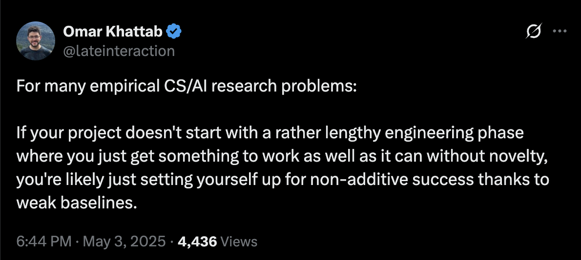
- Been making similar points myself.
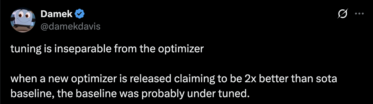
- I emphasized in my class on benchmarking optimizers, that one shouldn’t try to make such empirical claims unless one has the tuning budget of Google.
- My lecture on the deep learning tuning playbook discussed how to choose an initial baseline and then iteratively improve it: “hill climbing on baselines.”
- Theory papers should focus on finding the strongest baseline, too. If you look into the optimization literature, one might be surprised by how many do not improve any quantifiable metric, but instead develop a more “flexible and general method.” This is a problem with methods driven research. Some better ways to set the baseline in theory of optimization include showing your method provably:
- has a larger initialization region
- accelerates over sota in a neighborhood of the solution
- “works” for a class of problems where no principled method worked before
- has improved sample complexity or rate of convergence.
- reduces dependence on condition number while being implementable for specific empirical problems.
- does not require knowing certain unknowable problem parameters for implementation
- …
The ladder mechanism for ml competitions
TLDR
In the worst case, adapting models based on test set performance exponentially inflates generalization bounds; the ladder mechanism shows how to avoid this if we precommit to an adaptation rule.
The problem
Machine learning competitions use leaderboards to rank participants. Participants submit models $f_1, \dots, f_k$ iteratively. They receive scores $R_1, \dots, R_k$ based on performance on a held-out test set $S$. Participants use this feedback to create subsequent submissions $f_t$. This interaction creates an adaptive data analysis scenario where the analyst’s choices depend on information derived from the test set $S$. This adaptivity poses a challenge: standard statistical guarantees about model performance can fail. The empirical loss $R_S(f_t)$ computed on $S$ might not accurately reflect the true generalization loss $R_D(f_t)$, because $f_t$’s dependence on $S$ through past scores means $f_t$ is not independent of $S$. Participants might overfit the holdout set, leading to unreliable leaderboards. This work investigates this problem and introduces the ladder mechanism to maintain leaderboard reliability under such adaptive analysis.
Formalizing the problem and goal
The adaptive setting
The setup involves a holdout set $S = {(x_i, y_i)}_{i=1}^n$ drawn i.i.d. from a distribution $D$. We compute empirical loss $R_S(f) = \frac{1}{n} \sum_{i=1}^n l(f(x_i), y_i)$ and aim to understand the true loss $R_D(f) = \mathbb{E}_{(x,y) \sim D}[l(f(x), y)]$. The interaction proceeds sequentially: an analyst strategy $A$ generates $f_t$ based on history $(f_1, R_1, \dots, f_{t-1}, R_{t-1})$, and a leaderboard mechanism $L$ computes score $R_t$ using $f_t$, the history, and the sample $S$. The core difficulty is that $f_t$’s dependence on $S$ (via $R_{<t}$) breaks the independence assumption needed for standard statistical bounds.
Fixing the protocol
To analyze this adaptive process, the framework assumes the interaction protocol $(A, L)$ is fixed before the specific sample $S$ is drawn. The protocol includes the analyst’s deterministic algorithm $A$ for choosing $f_t$ and the host’s mechanism $L$ for computing $R_t$. This fixed protocol $(A, L)$ defines a conceptual tree $T$ representing all possible interaction histories. The set $F$ comprises all classifiers $f_t$ appearing at any node in this tree $T$. Importantly, $F$ is determined by the protocol $(A, L, k)$ and is fixed before the specific sample $S$ is used for evaluation.
leaderboard accuracy
The objective shifts from accurately estimating each $R_D(f_t)$ to ensuring the reported score $R_t$ accurately reflects the best true performance achieved up to step $t$. This is measured by the leaderboard error:
\[\text{lberr}(R_1, \dots, R_k) \overset{\text{def}}{=} \max_{1 \le t \le k} \left| \min_{1 \le i \le t} R_D(f_i) - R_t \right|\]The aim is to design a mechanism $L$ that minimizes this error against any analyst strategy $A$.
The ladder mechanism
The ladder mechanism is proposed as a simple algorithm for $L$. It controls the flow of information to the analyst by using a pre-defined step size $\eta > 0$.
The algorithm proceeds as follows:
- initialize the best score $R_0 = \infty$.
- for each round $t = 1, \dots, k$:
- receive classifier $f_t$ from the analyst $A$.
- compute the empirical loss $R_S(f_t)$ using the holdout set $S$.
- apply the decision rule: if $R_S(f_t) < R_{t-1} - \eta$, then update the reported score $R_t \leftarrow [R_S(f_t)]_\eta$. otherwise, maintain the previous score $R_t \leftarrow R_{t-1}$. (here, $[x]_\eta$ rounds $x$ to the nearest multiple of $\eta$.)
- report the score $R_t$ back to the analyst $A$.
The intuition behind the ladder is that it only reveals progress, i.e., a new, lower score, if the observed empirical improvement surpasses the threshold $\eta$. This quantization prevents the analyst from reacting to small fluctuations in $R_S(f)$ that might be specific to the sample $S$, thus limiting the leakage of information about $S$.
Theoretical upper bound
The ladder mechanism comes with a provable guarantee on its leaderboard accuracy.
theorem 3.1: for any deterministic analyst strategy $A$, the ladder mechanism $L$ using a step size $\eta = C \left( \frac{\log(kn)}{n} \right)^{1/3}$ (for a constant $C$) ensures that, with high probability over the draw of sample $S$ (of size $n$), the leaderboard error is bounded:
\[\text{lberr}(R_1, \dots, R_k) \le O\left( \left( \frac{\log(kn)}{n} \right)^{1/3} \right)\]This result is significant because the error depends only logarithmically on the number of submissions $k$. This implies robustness against prolonged adaptive interaction, contrasting with naive methods where error might grow polynomially with $k$.
Proof argument: uniform convergence over the function set $F$
The proof establishes that the empirical loss $R_S(f)$ converges uniformly to the true loss $R_D(f)$ over the entire set $F$ of functions potentially generated by the fixed protocol $(A, L)$.
- Bounding $|F|$ via compression (claim 3.2): The argument first bounds the size of $F$. The limited information release by the ladder mechanism restricts the complexity of the interaction tree $T$. Any node (representing a history and function $f_t$) in $T$ can be uniquely identified using a limited number of bits, $B$. This implies $|F| \le |T| \le 2^B$.
- Encoding scheme: to identify a node, we encode its path from the root. A path is characterized by the sequence of score updates. An “update step” at index $j$ occurs if $R_j < R_{j-1} - \eta$. The number of such steps along any path is at most $N_d \approx 1/\eta$. The number of possible score values $R_j$ at an update step is also bounded by $N_v \approx 1/\eta$. Encoding the indices and values of these update steps requires a certain number of bits. Claim 3.2 shows that $B = (1/\eta + 2)\log(4k/\eta)$ bits suffice.
- Bound: this yields $|F| \le 2^B$, where $B = O(\frac{1}{\eta}\log(k/\eta))$.
- Uniform convergence argument: Since $F$ is fixed before $S$ is observed, we can apply a uniform convergence argument using a union bound.
-
The probability that any function in $F$ has a large deviation is bounded:
\[\mathbb{P}\left\{ \exists f \in F : |R_S(f) - R_D(f)| > \epsilon \right\} \le \sum_{f \in F} \mathbb{P}\left\{ |R_S(f) - R_D(f)| > \epsilon \right\}\] -
For each fixed $f \in F$, Hoeffding’s inequality gives
\[\mathbb{P}\{|R_S(f) - R_D(f)| > \epsilon\} \le 2e^{-2\epsilon^2 n}.\] -
Combining these yields the overall failure probability bound:
\[\mathbb{P}\{\text{large deviation in } F\} \le |F| \cdot 2e^{-2\epsilon^2 n} \le 2 \cdot 2^B e^{-2\epsilon^2 n}\]
-
-
Balancing error terms: We need this probability to be small. This requires the exponent to be sufficiently negative, essentially $2\epsilon^2 n \gtrsim B \approx \frac{1}{\eta}\log(k/\eta)$. The total leaderboard error comprises statistical error $\epsilon$ and mechanism threshold error $\eta$, totaling approximately $\epsilon + \eta$. To minimize this sum subject to the constraint $2\epsilon^2 n \approx \frac{1}{\eta}\log(k/\eta)$, we balance the terms, leading to $\epsilon \approx \eta$. Substituting back into the constraint yields $2\eta^3 n \approx \log(k/\eta)$. This resolves to $\eta \approx \epsilon \approx \left( \frac{\log(k/\eta)}{n} \right)^{1/3}$. Choosing $\eta = O\left( \left( \frac{\log(kn)}{n} \right)^{1/3} \right)$ makes the failure probability small.
- Implication for leaderboard error: The uniform convergence ensures that, with high probability, $|R_S(f) - R_D(f)| \le \epsilon$ holds simultaneously for all $f \in F$. Since the actual sequence $f_1, \dots, f_k$ must belong to $F$, this guarantee applies to them. This property, combined with the ladder’s update rule (which relates $R_t$ to $R_S(f)$ for some $f$ that triggered an update), allows proving that the reported score $R_t$ stays within $\approx \epsilon + \eta$ of the true best score $\min_{i \le t} R_D(f_i)$. This bounds the leaderboard error as stated in the theorem.
Theoretical lower bound
The paper also establishes a fundamental limit on the accuracy achievable by any leaderboard mechanism.
theorem 3.3: For any mechanism $L$, there exist scenarios (distributions $D$, classifiers $f_i$) where the expected worst-case leaderboard error is bounded below:
\[\inf_L \sup_D \mathbb{E}_S[\text{lberr}(R(S))] \ge \Omega\left( \sqrt{\frac{\log k}{n}} \right)\]This lower bound highlights a gap between the ladder’s $n^{-1/3}$ performance and the optimal $n^{-1/2}$ dependence. The proof utilizes a reduction to high-dimensional mean estimation combined with Fano’s inequality.
Practical stuff
Parameter-free ladder mechanism
A practical challenge is setting the step size $\eta$ without prior knowledge of $k$ and $n$. A parameter-free variant addresses this by adapting the threshold dynamically.
- it maintains the best score $R_{t-1}$ and the loss vector $l_{prev}$ of the submission that achieved it.
- for a new submission $f_t$ with loss vector $l_t$, it computes the sample standard deviation $s = \text{std}(l_t - l_{prev})$.
- it uses an adaptive threshold $\eta_t = s/\sqrt{n}$.
- the update rule becomes: update $R_t \leftarrow [R_S(f_t)]_{1/n}$ if $R_S(f_t) < R_{t-1} - \eta_t$. otherwise, $R_t \leftarrow R_{t-1}$. This approach uses a heuristic related to a paired t-test to gauge statistical significance based on observed variance.
The boosting attack
This attack demonstrates the weakness of leaderboard mechanisms that reveal empirical scores with high precision.
- it targets mechanisms where the reported score $R_t$ is very close to $R_S(f_t)$.
- the attack proceeds by submitting $k$ random classifiers $u_i$ and observing their scores $l_i \approx R_S(u_i)$. it identifies a subset $I$ of classifiers that performed slightly better than chance on $S$ (e.g., $l_i \le 1/2$). a final classifier $u^*$ is formed by taking a majority vote over this subset ${u_i : i \in I}$.
- if the score precision is high (error significantly less than $1/\sqrt{n}$), the attack can yield $u^*$ with $R_S(u^* ) \ll 1/2$ but $R_D(u^* ) \approx 1/2$. this creates a large leaderboard error, $\Omega(\sqrt{k/n})$. the ladder mechanism resists this attack because its threshold $\eta \approx n^{-1/3}$ is much coarser than the $n^{-1/2}$ precision needed for the attack to reliably identify the slightly advantageous random classifiers. it simply doesn’t provide precise enough feedback.
What is kv cache?
\[\begin{aligned} \textbf{(1) Projections:}\quad & q = W_Q x_{t+1},\; k = W_K x_{t+1},\; v = W_V x_{t+1};\\[2mm] % \textbf{(2) Cache append:}\quad & K_{1:t+1} = \begin{bmatrix} K_{1:t}\\ k \end{bmatrix},\; V_{1:t+1} = \begin{bmatrix} V_{1:t}\\ v \end{bmatrix};\\[2mm] % \textbf{(3) New logit:}\quad & s_{t+1} = \frac{1}{\sqrt{d}}\;q k^{\top},\qquad e_{t+1} = e^{s_{t+1}};\\[2mm] % \textbf{(4) Incremental softmax:}\quad & Z_{t+1} = Z_{t} + e_{t+1},\\ &\alpha_i^{(t+1)} = \alpha_i^{(t)}\frac{Z_{t}}{Z_{t+1}}\;\;(1\le i\le t),\qquad \alpha_{t+1}^{(t+1)} = \frac{e_{t+1}}{Z_{t+1}};\\[2mm] % \textbf{(5) Output:}\quad & z_{t+1} = \sum_{i=1}^{t+1} \alpha_i^{(t+1)} v_i = \alpha^{(t+1)} V_{1:t+1}. \end{aligned}\]What is constitutional AI?
Constitutional ai trains harmless ai using ai feedback, guided by principles (a ‘constitution’), instead of human harm labels.
- Supervised phase (initial training):
- Generate: get initial responses from a helpful-only model. purpose: create raw examples.
- Critique: ai identifies harm in responses using the constitution. purpose: find flaws based on principles.
- Revise: ai rewrites responses to remove harm, guided by critique. purpose: create corrected examples.
- Finetune: train the model on the ai-revised responses. purpose: teach the model initial harmlessness.
- Reinforcement learning phase (refinement):
- Generate pairs: the supervised model creates pairs of responses to prompts. purpose: provide choices for comparison.
- Evaluate: ai chooses the less harmful response based on the constitution. purpose: create preference data without human labels.
- Train preference model (pm): build a model predicting ai preferences. purpose: capture the constitution as a reward signal.
- Reinforce: train the supervised model using the pm’s score as a reward. purpose: optimize the ai for constitutional alignment.
this process uses ai oversight, defined by a constitution, to scale alignment and reduce reliance on direct human judgment for harmfulness.
Multi head, multi query, and grouped query attention
\[X\in\mathbb{R}^{T\times d},\qquad d = H\,d_k,\qquad {\rm softmax}(S)_{ij} = \exp(S_{ij}) \big/ \textstyle\sum_{m}\exp(S_{im}).\]Multi-head attention (MHA)
The total number of K/V heads is H \(\begin{aligned} (1)\;& Q_h = X W_{Q,h},\; K_h = X W_{K,h},\; V_h = X W_{V,h}; \\[2pt] (2)\;& S_h = \tfrac{1}{\sqrt{d_k}}\,Q_h K_h^{\top}; \\[2pt] (3)\;& \alpha_h = {\rm softmax}(S_h); \\[2pt] (4)\;& Z_h = \alpha_h V_h; \\[2pt] (5)\;& Z = \bigl[Z_1\;\Vert\;\dots\;\Vert\;Z_H\bigr]\,W_O. \\[4pt] \text{Cache size: }&2\,H\,T\,d_k \quad(\text{keys+values}). \end{aligned}\)
Multi-query attention (MQA)
The total number of K/V heads is 1 \(\begin{aligned} (1)\;& Q_h = X W_{Q,h},\qquad K = X W_K,\qquad V = X W_V; \\[2pt] (2)\;& S_h = \tfrac{1}{\sqrt{d_k}}\,Q_h K^{\top}; \\[2pt] (3)\;& \alpha_h = {\rm softmax}(S_h),\qquad Z_h = \alpha_h V; \\[2pt] (4)\;& Z = \bigl[Z_1\;\Vert\;\dots\;\Vert\;Z_H\bigr]\,W_O. \\[4pt] \text{Cache size: }&2\,T\,d_k \quad(\text{$H$-fold reduction}). \end{aligned}\)
Grouped-query attention (GQA)
The total number of K/V heads is G, where 1 < G < H \(\begin{aligned} (1)\;& \text{partition heads into groups }g=1,\dots,G\ \text{of size }H/G; \\[2pt] (2)\;& Q_h = X W_{Q,h},\; K_g = X W_{K,g},\; V_g = X W_{V,g}\quad(h\in g); \\[2pt] (3)\;& S_h = \tfrac{1}{\sqrt{d_k}}\,Q_h K_g^{\top}; \\[2pt] (4)\;& \alpha_h = {\rm softmax}(S_h),\qquad Z_h = \alpha_h V_g; \\[2pt] (5)\;& Z = \bigl[Z_1\;\Vert\;\dots\;\Vert\;Z_H\bigr]\,W_O. \\[4pt] \text{Cache size: }&2\,G\,T\,d_k \quad(\text{$H/G$-fold reduction}). \end{aligned}\)
Purpose
Smaller #K/V heads $\;\Rightarrow\;$ smaller KV-cache $\;\Rightarrow\;$ lower memory-bandwidth during autoregressive decoding, hence higher tokens per second. Quality degrades monotonically with the reduction factor; $G$ is a hardware–quality dial.