Scaling Transformers: Parallelism Strategies from the Ultrascale Playbook
Resources
Visualizations
Visualization for DP, FSDP, and TP
Minimalist 0-6D Parallelism from Main Horse
Blogs/books
Ultrascale Playbook (main source for this lecture)
Lilian Weng’s blog: How to Train Really Large Models on Many GPUs?
Table of Contents
- Introduction: The Scaling Challenge
- Transformers: Anatomy of a Large Model
- The Memory Bottleneck: Activations in Backpropagation
- Activation Recomputation (Gradient Checkpointing)
- Primer: Distributed Communication Primitives
- Parallelism Strategies
- Combining Strategies & Conclusion
1. Introduction: The Scaling Challenge
Modern Transformer models frequently contain billions or even trillions of parameters. Training these large models presents significant computational challenges, particularly concerning GPU memory, which often exceeds the capacity of a single accelerator device. This necessitates distributed training, distributing the workload across multiple devices.
This lecture focuses on the system-level challenges and practical strategies for distributing the training process, moving beyond the specifics of optimization algorithms covered previously. We will draw heavily on the insights and techniques detailed in the Hugging Face Ultrascale Playbook (available here), a key resource for scaling Transformer training.
We will begin by reviewing the Transformer architecture to pinpoint sources of high computational and memory demands. Subsequently, we identify activation memory as a primary bottleneck during backpropagation and introduce activation recomputation as a crucial memory-saving technique. A primer on essential distributed communication primitives follows, providing the foundation for understanding parallelism. The core of the lecture analyzes the main parallelism strategies outlined in the playbook: Data Parallelism (DP), including its memory-efficient variants like ZeRO/Fully Sharded Data Parallelism (FSDP); Tensor Parallelism (TP) and its enhancement, Sequence Parallelism (SP); Context Parallelism (CP) for long sequences; Pipeline Parallelism (PP) with its scheduling considerations; and Expert Parallelism (EP) for Mixture-of-Experts models. Finally, we discuss how these strategies are combined in practice and conclude with guidance on selecting appropriate configurations.
Note: I wrote this guide for my students after reading through the Ultrascale Playbook by myself. The content is essentially a subset of what is covered in the playbook, but I added supporting detail where I struggled to understand concepts. I am grateful to the authors for writing this document and allowing me to include their figures in these notes.
2. Transformers: Anatomy of a Large Model
This section introduces the essential structure of the standard Transformer model. The objective is to identify the components responsible for the model’s large parameter count and computational cost, which are critical factors for understanding parallelism strategies. This overview is not exhaustive; for a detailed visual and interactive exploration of the Transformer architecture, the “Transformer Explainer” (available here) provides an excellent resource. Readers unfamiliar with the basic mechanism should review it.
A Transformer model processes a sequence of input tokens, typically represented as integer indices $x = (x_1, \dots, x_s)$, where $s$ is the sequence length. The overall computation involves an initial embedding layer, followed by a stack of $L$ identical Transformer Blocks, and usually concludes with a task-specific output layer (e.g., projecting to vocabulary logits for language modeling).
The Embedding Layer maps the input token indices $x$ to a sequence of continuous vectors $H^{(0)} \in \mathbb{R}^{s \times h}$, where $h$ is the hidden dimension of the model. This is done using a learnable token embedding matrix $W_E \in \mathbb{R}^{V_{size} \times h}$, where $V_{size}$ is the vocabulary size. Each token $x_i$ is mapped to its corresponding row vector in $W_E$. Positional information is then added, typically using fixed or learned positional encodings $P \in \mathbb{R}^{s \times h}$. The resulting initial representation is:
\[H^{(0)} = \text{Embed}(x) + P\]where $\text{Embed}(x)_i = W_E[x_i, :]$ denotes taking the $x_i$-th row of $W_E$. The parameters in this initial stage reside primarily in the embedding matrix $W_E$.
Before describing the Transformer Block, we define Layer Normalization (LN), a technique used throughout the model to stabilize training. Given an input tensor $Z \in \mathbb{R}^{s \times h}$, LN normalizes the activations independently for each token (row) $i$ across the hidden dimension $h$. For the $i$-th token vector $Z_i \in \mathbb{R}^h$, the computation is:
\[\text{LN}(Z)_i = \gamma \odot \frac{Z_i - \mu_i}{\sqrt{\sigma_i^2 + \epsilon}} + \beta\]Here, $\mu_i = \frac{1}{h}\sum_{j=1}^h Z_{ij}$ and $\sigma_i^2 = \frac{1}{h}\sum_{j=1}^h (Z_{ij} - \mu_i)^2$ are the mean and variance computed across the hidden dimension $h$ for token $i$. The parameters $\gamma \in \mathbb{R}^h$ and $\beta \in \mathbb{R}^h$ are learnable scale and shift parameters, respectively, and $\epsilon$ is a small constant (e.g., $10^{-5}$) added for numerical stability. The symbol $\odot$ denotes element-wise multiplication. Each LN layer adds $2h$ learnable parameters.
The core of the Transformer consists of $L$ stacked Transformer Blocks. Each block $l$ takes an input $H^{(l-1)} \in \mathbb{R}^{s \times h}$ (starting with $H^{(0)}$) and produces an output $H^{(l)} \in \mathbb{R}^{s \times h}$. Within each block, there are two main sub-layers: Multi-Head Self-Attention (MHA) and a Position-wise Feedforward Network (FFN). Residual connections and Layer Normalization are applied around these sub-layers. We describe the common Pre-LN variant, where LN is applied before the input enters each sub-layer.
The Multi-Head Attention (MHA) sub-layer allows the model to weigh information from different positions in the sequence.
- First, the input is normalized: $X’ = \text{LN}_1(H^{(l-1)})$.
-
This normalized input $X’$ is linearly projected to generate Queries (Q), Keys (K), and Values (Val) using learnable weight matrices $W_Q, W_K, W_V \in \mathbb{R}^{h \times h}$:
\[Q = X' W_Q, \quad K = X' W_K, \quad Val = X' W_V\] - To form $a$ attention heads, the resulting $Q, K, Val$ matrices (each in $\mathbb{R}^{s \times h}$) are conceptually split along the hidden dimension into $a$ smaller matrices $Q_i, K_i, Val_i \in \mathbb{R}^{s \times d_k}$, where the head dimension is $d_k = h/a$. This corresponds to partitioning the weight matrices $W_Q, W_K, W_V$.
-
For each head $i$, scaled dot-product attention is computed:
\[\text{Scores}_i = \text{softmax}_{\text{keys}}\left(\frac{Q_i K_i^T}{\sqrt{d_k}}\right) \in \mathbb{R}^{s \times s}\]The $\text{softmax}_{\text{keys}}$ function is applied row-wise to the $s \times s$ matrix of dot products. For a row $z$ of the input matrix, $(\text{softmax}(z))_j = e^{z_j} / \sum_{p=1}^{s} e^{z_p}$, normalizing the attention weights across all key positions for each query position.
-
The output for head $i$ is a weighted sum of Value vectors:
\[O_i = \text{Scores}_i \cdot Val_i \in \mathbb{R}^{s \times d_k}\] -
The outputs of all heads are concatenated back together:
\[O_{concat} = \text{Concat}(O_1, \dots, O_a) \in \mathbb{R}^{s \times h}\] -
Finally, the concatenated outputs are projected using another learnable weight matrix $W_O \in \mathbb{R}^{h \times h}$:
\[O_{MHA} = O_{concat} W_O\]
The parameters for the MHA sub-layer are $W_Q, W_K, W_V, W_O$ (and associated biases, often omitted for simplicity or absorbed). The primary computations involve the initial projections, the $QK^T$ matrix multiplication, the $\text{Scores} \cdot Val$ matrix multiplication, and the final projection $W_O$.
After the MHA computation, a Residual Connection adds the original input to the MHA output:
\[H_{intermediate} = H^{(l-1)} + O_{MHA}\]The Position-wise Feedforward Network (FFN) sub-layer then processes this intermediate result.
- First, the input is normalized: $X’’ = \text{LN}_2(H_{intermediate})$.
-
The FFN applies two linear transformations with a non-linearity (commonly GELU) in between:
\[O_{FFN} = \text{GELU}(X'' W_1 + b_1) W_2 + b_2\]Here, $W_1 \in \mathbb{R}^{h \times d_{ff}}$ and $b_1 \in \mathbb{R}^{d_{ff}}$ are parameters for the first linear layer, and $W_2 \in \mathbb{R}^{d_{ff} \times h}$ and $b_2 \in \mathbb{R}^{h}$ are for the second. The intermediate dimension $d_{ff}$ is typically larger than $h$, often $d_{ff}=4h$. The parameters are $W_1, b_1, W_2, b_2$. The computation is dominated by the two large matrix multiplications involving $W_1$ and $W_2$.
A second Residual Connection adds the input to the FFN sub-layer to its output, producing the final output of the Transformer block $l$:
\[H^{(l)} = H_{intermediate} + O_{FFN}\]After the final block $L$, the output $H^{(L)}$ is often normalized one last time:
\[H'_{final} = \text{LN}_{final}(H^{(L)}).\]An Output Layer then typically projects this final representation to the desired output space. For language modeling, this involves a linear layer with weights $W_{LM} \in \mathbb{R}^{h \times V_{size}}$ (often sharing weights with $W_E$):
\[\text{Logits} = H'_{final} W_{LM} \in \mathbb{R}^{s \times V_{size}}\]The entire Transformer model $f$, parameterized by weights $w$, maps an input sequence $x$ to output logits:
\[f(x; w) = \text{OutputLayer} \circ \text{Block}_L \circ \dots \circ \text{Block}_1 \circ \text{EmbeddingLayer}(x)\]Training optimizes the parameters $w$ by minimizing an objective function $L(w)$, typically the expected loss over a data distribution, $L(w) = \mathbb{E}_z[\ell(w, z)]$. The loss $\ell(w, z)$ is computed for individual data samples $z$. For autoregressive language modeling, a data sample $z = (x, y)$ consists of an input sequence $x = (x_1, \dots, x_s)$ and a target sequence $y = (y_1, \dots, y_s)$, where $y_t = x_{t+1}$ represents the token following $x_t$. The standard loss function is the Cross-Entropy Loss, calculated between the model’s predicted logit distribution and the actual target token index at each sequence position $t$:
\[\ell(w, z) = -\frac{1}{s} \sum_{t=1}^{s} \log P(y_t | x_1, \dots, x_t; w)\]The probability $P(y_t | x_1, \dots, x_t; w)$ is derived from the model’s output logits $\text{Logits} = f(x; w) \in \mathbb{R}^{s \times V_{size}}$. Specifically, for position $t$, let $\text{Logits}_t \in \mathbb{R}^{V_{size}}$ be the logit vector. The probability of observing vocabulary item $v$ is:
\[P(v | x_1, \dots, x_t; w) = \frac{\exp(\text{Logits}_{t,v})}{\sum_{v'=1}^{V_{size}} \exp(\text{Logits}_{t,v'})}\]Minimizing the objective $L(w)$ requires computing gradients with respect to all parameters $w$ and updating them. Therefore, understanding the location and scale of these parameters, as well as the computational cost of the forward and backward passes through the architecture defined above, is essential for developing efficient scaling strategies.
In summary, the parameters in a standard Transformer model are concentrated in the embedding matrix $W_E$, the MHA projection matrices ($W_Q, W_K, W_V, W_O$ per layer), the FFN weights ($W_1, W_2$ per layer), the LN parameters ($\gamma, \beta$ per normalization), and the final output projection matrix $W_{LM}$. The computational cost is dominated by the large matrix multiplications performed within the MHA mechanism ($QK^T$, $\text{Scores} \cdot Val$) and the FFN layers ($XW_1$, $HW_2$), repeated across $L$ blocks. Understanding this distribution is crucial for designing effective parallelism strategies.
Common Modifications: Attention Masking and Dropout
The structure described above represents a standard Transformer block. Two common modifications are frequently incorporated for specific modeling purposes or regularization during training: Attention Masking and Dropout.
Attention Masking controls which key positions each query position can attend to. This is necessary for tasks like autoregressive language modeling, where a token should not attend to future tokens. Masking is typically implemented by adding a mask matrix $M \in {0, -\infty}^{s \times s}$ to the scaled dot-product scores before the softmax operation:
\[\text{Scores}_i = \text{softmax}_{\text{keys}}\left(\frac{Q_i K_i^T}{\sqrt{d_k}} + M\right) \in \mathbb{R}^{s \times s}\]Where $M_{jk} = -\infty$, the exponentiated value becomes zero, effectively preventing attention from query position $j$ to key position $k$. A common causal mask sets $M_{jk} = -\infty$ for all $k > j$ and $M_{jk} = 0$ otherwise. This ensures that position $j$ attends only to positions $k \le j$. Other mask patterns can be used, for example, to ignore padding tokens.
Dropout is a regularization technique used during training to prevent overfitting. It randomly sets a fraction $p$ (the dropout probability) of elements in an input tensor to zero and scales the remaining elements by $1/(1-p)$ to maintain the expected value. Dropout is typically applied after the attention output projection ($O_{MHA}$) and after each linear layer within the FFN. Mathematically, during training for an input $Z$:
\[\text{Dropout}(Z)_{train} = \frac{1}{1-p} \cdot (Z \odot B)\]where $B$ is a binary mask tensor with elements randomly set to 0 (with probability $p$) or 1 (with probability $1-p$), drawn independently for each training step. During inference, Dropout is deactivated, effectively becoming an identity function ($\text{Dropout}(Z)_{inference} = Z$). The only parameter is the dropout rate $p$.
3. The Memory Bottleneck: Activations in Backpropagation
PyTorch relies on autodifferentiation (e.g., the formal chain rule) to compute gradients of the loss function $\ell(w, z)$ with respect to the model parameters $w$. Autodifferentiation, or backpropagation as it’s called in the deep learning literature, operates by applying the chain rule recursively, starting from the output layer and moving backward through the network. A key requirement of this process is access to intermediate values computed during the forward pass. These intermediate values are often referred to collectively as “activations.” Storing these activations consumes significant memory, often becoming the primary bottleneck when training large models. (See Lectures 4 and 5 for background on computational graphs and automatic differentiation).
Specifically, to compute the gradient with respect to the parameters of a given layer (e.g., the weights $W$ in a linear layer $Y = XW$), backpropagation typically requires the input to that layer during the forward pass (e.g., $X$). Furthermore, to compute the gradient of the loss with respect to the input of that layer (needed to propagate gradients further back), one often needs intermediate results computed within that layer (e.g., the output $Y$ or values computed before a non-linearity). Therefore, many intermediate tensors generated during the forward pass must be stored until they are used in the corresponding backward pass computation.
The total memory required to store these necessary activations depends on several factors related to the model architecture and the training configuration. Key factors include:
- The batch size (
b): The number of independent sequences processed in parallel. - The sequence length (
s): The number of tokens in each input sequence. - The hidden dimension (
h): The size of the representation vectors within the model. - The number of layers (
L): The depth of the model. - Model-specific dimensions like the feedforward intermediate dimension (
d_ff). - The data type used for activations (e.g., float32, float16, bfloat16).
Consider a single transformer block. The input and output tensors $H^{(l-1)}$ and $H^{(l)}$ have dimensions $s \times h$. If processing a batch of size $b$, these tensors become $b \times s \times h$. Many intermediate computations within the MHA and FFN sub-layers (e.g., $Q, K, Val$, attention scores, FFN hidden states) also have dimensions proportional to $b, s, h,$ or $d_{ff}$. Storing these intermediate results across all $L$ layers leads to a total activation memory requirement that scales approximately as:
\[\text{Activation Memory} \approx C \times L \times b \times s \times h \times (\text{bytes per element})\]The constant $C$ depends on the specific transformer architecture and which intermediate values are stored for the backward pass. For standard transformers, $C$ can be significant because values like the attention scores ($b \times a \times s \times s$) or the intermediate FFN activations ($b \times s \times d_{ff}$) must often be kept.
It is crucial to contrast this with the memory required for model parameters. The number of parameters scales primarily with the number of layers $L$ and dimensions related to the model’s width, such as the hidden dimension $h$ and the intermediate feedforward dimension $d_{ff}$. Key parameter matrices include the token embeddings ($W_E \in \mathbb{R}^{V_{size} \times h}$), the attention projections ($W_Q, W_K, W_V, W_O \in \mathbb{R}^{h \times h}$ per layer), the FFN weights ($W_1 \in \mathbb{R}^{h \times d_{ff}}, W_2 \in \mathbb{R}^{d_{ff} \times h}$ per layer), and potentially a final output projection ($W_{LM} \in \mathbb{R}^{h \times V_{size}}$). The total parameter memory is approximately:
\[\begin{aligned} &\text{Parameter Memory} \\ &\approx (\text{Size}(W_E) + \text{Size}(W_{LM}) + L \times (\text{Size}(W_{Q,K,V,O}) + \text{Size}(W_{1,2}) + \text{Size}(\gamma, \beta)_{\text{LN}})) \\ &\hspace{20pt} \times (\text{bytes per element}) \end{aligned}\]Assuming $d_{ff}=4h$ and shared embedding/output weights ($W_{LM} \approx W_E^T$), this scales roughly as $O(V_{size}h + L h^2)$. The critical difference lies in the dependence on batch size b and sequence length s. Parameter memory is independent of these factors, while activation memory grows linearly with both. In large-scale transformer training, where large batch sizes are used for efficiency and sequences can be long, the activation memory often dwarfs the parameter memory. This makes activation storage the primary constraint limiting the size of the model or the batch size that can fit onto a single accelerator device. Techniques to manage this activation memory are therefore essential for scaling transformer training.
4. Activation Recomputation (Gradient Checkpointing)
Activation recomputation, also commonly known as gradient checkpointing, is a technique designed specifically to alleviate the activation memory bottleneck described in Section 3. The core idea is to trade increased computation time for reduced memory usage (Note: as Horace He mentions, “In the presence of a fusing compiler, recomputation can actually reduce both memory and runtime.”). Instead of storing all intermediate activations computed during the forward pass that are needed for the backward pass, only a strategically chosen subset of activations is saved. During the backward pass, whenever an activation is required but was not stored, it is recomputed on-the-fly by performing a partial forward pass starting from the nearest previously stored activation. (Playbook, Section: activation_recomputation).
For example, within a transformer model, one might choose to store only the inputs to each transformer block ($H^{(l-1)}$) and discard all activations computed inside the block (e.g., intermediate MHA and FFN results). When the backward pass needs these internal activations to compute gradients for the block’s parameters, the block’s forward computation is executed again, starting from the stored $H^{(l-1)}$, to regenerate the needed values just before they are used. This avoids storing the potentially large intermediate tensors from MHA and FFN throughout the entire forward and backward pass of the whole network.
The trade-off is clear: memory usage is significantly reduced because fewer intermediate tensors are stored, but computational cost increases because parts of the forward pass are executed twice (once during the initial forward pass, and again during the backward pass for recomputation). The typical increase in compute time is roughly equivalent to performing one extra forward pass for the segments where recomputation is applied. Activation recomputation is often essential for training very large models or for utilizing larger effective batch sizes than would otherwise fit within the available device memory.
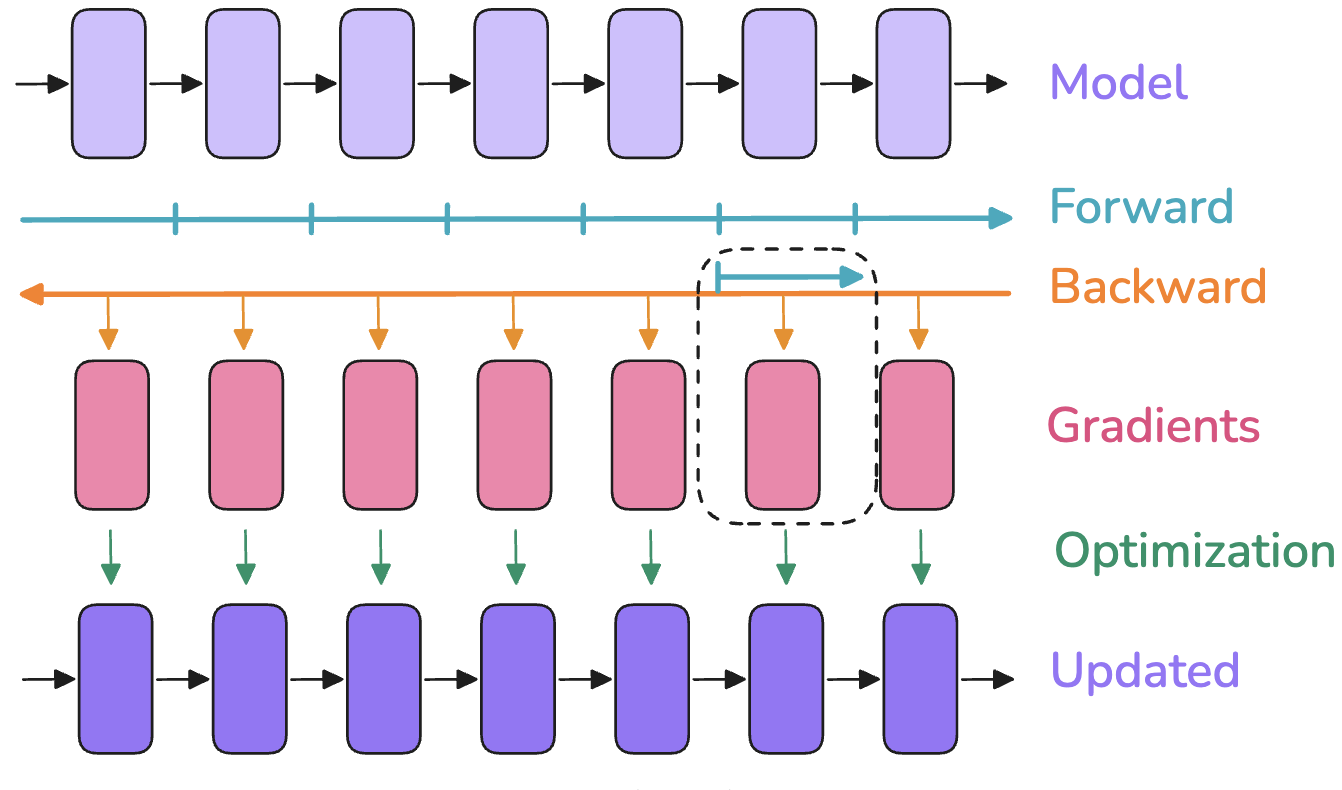 Figure 1: Activation Recomputation. Recomputation trades compute for memory by recomputing intermediate activations during the backward pass. The top shows a standard forward and backward pass where all activations are stored. The bottom shows activation recomputation where only the input to the recomputed segment is stored, and activations within the segment are recomputed during the backward pass. [Playbook, Section: activation_recomputation])
5. Primer: Distributed Communication Primitives
Distributing model training across multiple devices, such as gpus, necessitates communication between these independent processing units, often referred to as workers. Standard patterns for this inter-worker communication and synchronization are known as collective operations. Understanding these basic operations is essential for grasping how different parallelism strategies function. This section provides a brief overview of common communication primitives, drawing from the concepts outlined in the Ultrascale Playbook appendix (Playbook, Appendix A0: Parallel Programming Crash Course).
We consider a group of $N$ workers involved in the distributed computation. Each worker is assigned a unique integer identifier, its rank, typically ranging from $0$ to $N-1$. Some collective operations involve a designated root worker, or specify source (src) and destination (dst) ranks for the data transfer.
The Broadcast operation involves one designated source worker (src) sending an identical copy of its data tensor to all other workers in the group, including itself. This is commonly used to distribute initial model parameters or configuration settings from one worker (e.g., rank 0) to all others at the beginning of training.
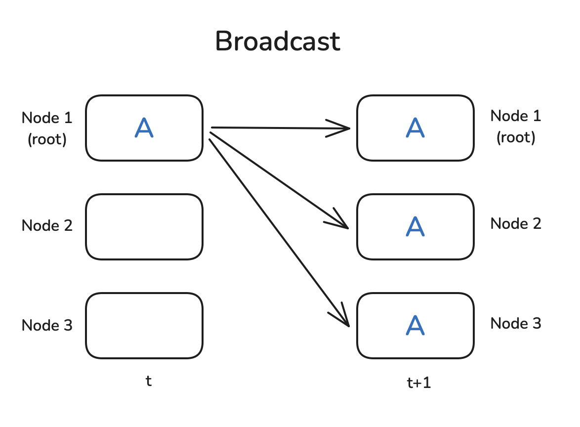 Figure 2: Broadcast Operation (Playbook, Section: broadcast)
The Reduce operation aggregates data from all workers. Each worker provides an input tensor, and a specified reduction function (e.g., SUM, AVG, MAX, MIN) is applied element-wise across these input tensors. The final tensor containing the reduced result is stored only on a single, designated destination worker (dst). This allows, for example, summing partial results computed across workers onto one main worker.
The AllReduce operation also performs an element-wise reduction across input tensors from all workers, using a specified function like SUM. However, unlike Reduce, the final reduced tensor result is then distributed back to all workers in the group. This primitive is fundamental to Data Parallelism (discussed in Section 6.1), where it is used to average the gradients computed independently on each worker.
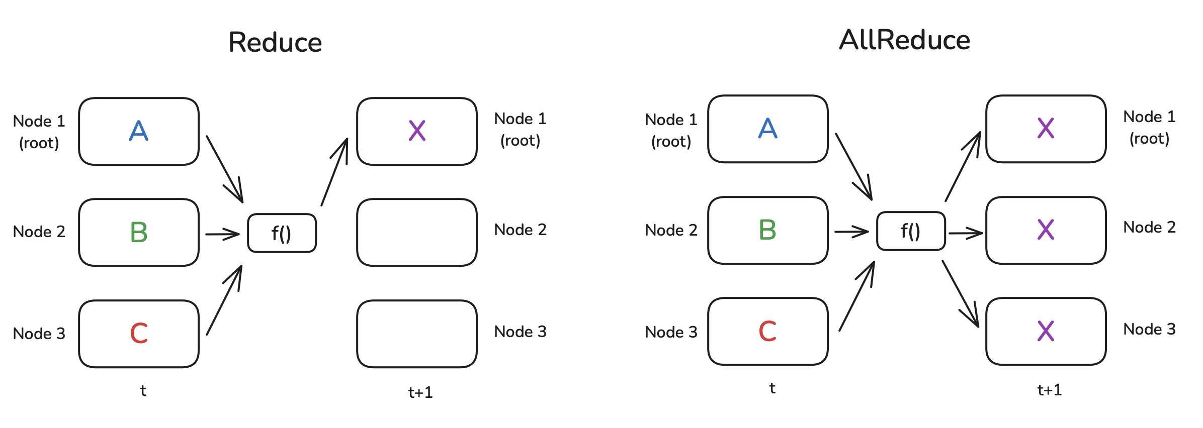 Figure 3: Reduce and AllReduce Operations (Playbook, Section: Reduce and AllReduce)
The Gather operation collects distinct data chunks from different workers onto a single worker. Each worker $k$ initially holds its own tensor $T_k$. In a Gather operation, all these tensors $T_0, T_1, …, T_{N-1}$ are sent to a designated destination worker (dst), which then holds the collection of all tensors (e.g., concatenated or as a list).
The AllGather operation performs the same collection process as Gather, gathering the distinct tensor $T_k$ from each worker $k$. However, the resulting collection of all tensors $(T_0, …, T_{N-1})$ is made available to all workers in the group, not just the destination worker. This is useful when all workers need access to the complete set of data distributed across the group, such as gathering sharded parameters in certain parallelism schemes.
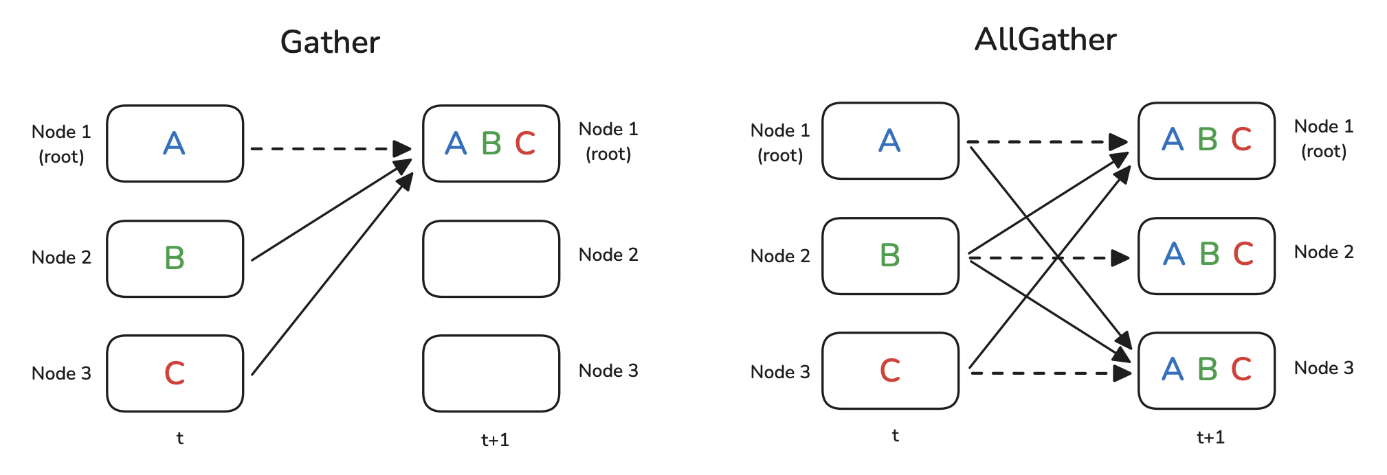 Figure 4: Gather and AllGather Operations (Playbook, Section: Gather and AllGather)
The Scatter operation is functionally the inverse of Gather. A single designated source worker (src) holds a collection of distinct data chunks (e.g., a list of tensors or a partitioned tensor). It sends exactly one distinct chunk to each worker in the group, including itself. This distributes different pieces of data from one source to multiple destinations.
The ReduceScatter operation combines aggregation and scattering. Each worker $k$ starts with a collection of data chunks, where chunk $j$ is notionally intended for worker $j$. First, for each chunk index $j$, the corresponding chunks from all workers are reduced together (e.g., summed element-wise). Then, the resulting reduced chunk $j$ is sent only to worker $j$. This is used, for instance, in Fully Sharded Data Parallelism (Section 6.4) to compute and distribute shards of the averaged gradients efficiently.
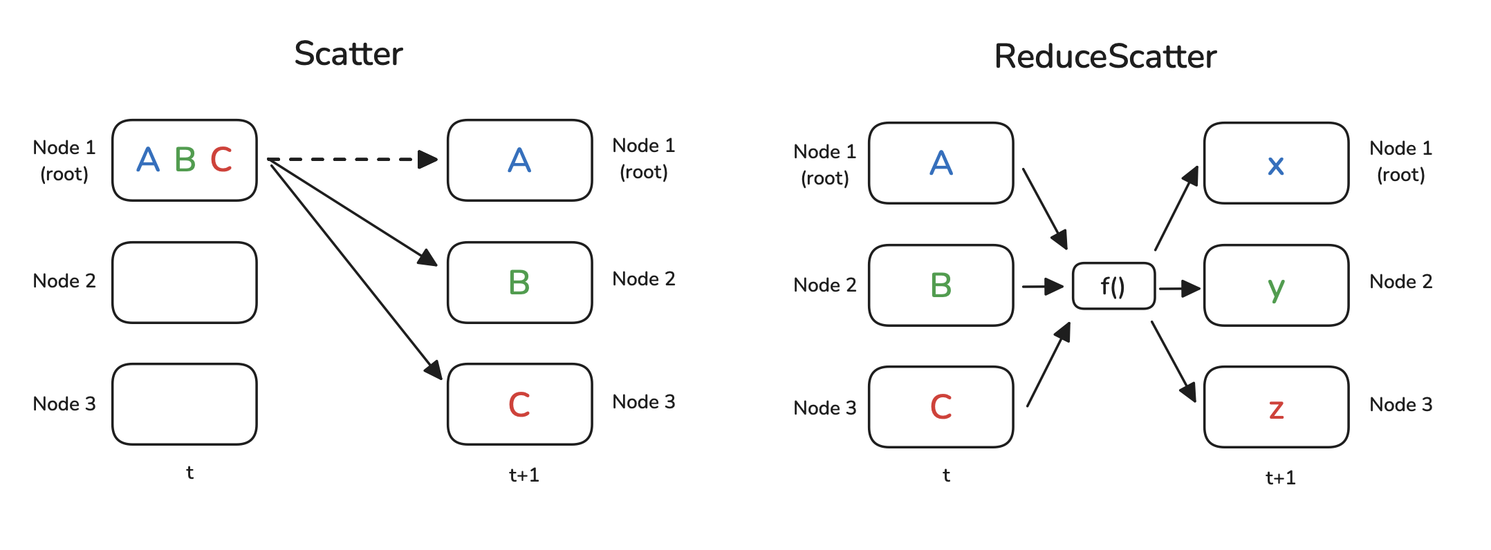 Figure 5: Scatter and ReduceScatter Operations (Playbook, Section: Scatter and ReduceScatter)
The Barrier operation provides explicit synchronization. When a worker calls barrier, it pauses execution until all other workers in the group have also called barrier. Once all workers have reached the barrier, they are all allowed to proceed. This ensures that certain stages of computation are complete across all workers before the next stage begins, although excessive use can introduce unnecessary delays by forcing faster workers to wait for slower ones.
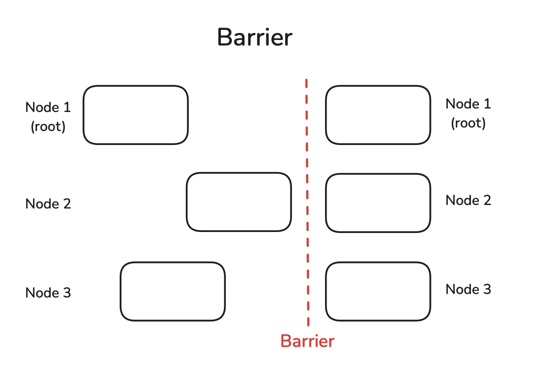 Figure 6: Barrier Operation (Playbook, Section: barrier)
These collective operations are typically implemented in specialized communication libraries. For distributed GPU training, the NVIDIA Collective Communications Library (NCCL) is widely used. NCCL provides highly optimized implementations of these primitives for efficient communication directly between GPUs, often leveraging high-speed interconnects like NVLink. Frameworks like PyTorch utilize NCCL as a backend to perform these distributed communication tasks during training.
6. Parallelism Strategies
Having established the structure of large transformer models, the activation memory bottleneck, and the utility of activation recomputation, we now turn to the primary strategies used to distribute the training workload across multiple accelerator devices. These techniques, detailed in the Hugging Face Ultrascale Playbook, allow us to overcome the memory and compute limitations of a single device by partitioning the model state and computation in different ways.
Note: I’ve made a little visualization of data parallelism, fully sharded data parallelism, and transformer parallelism, which you can view here. There are some small errors in the visualization, but it should more or less give you the idea. It was an absolute nightmare to make. I tried every model/coding tool that was available on Friday April 17th, 2025, but only with claude code was able to make something that was somewhat satisfactory.
6.1 Data Parallelism (DP)
Data Parallelism (DP) is a widely used strategy where the complete set of model parameters, denoted by $w$, is replicated on each of $N_d$ participating worker devices (e.g., gpus) in a DP group. Training involves processing a large global data batch $\mathcal{B}$. This batch is divided into $N_d$ smaller micro-batches, $\mathcal{B}_k$, where $k \in {1, \dots, N_d}$. Each worker $k$ independently performs the forward pass using its local micro-batch $\mathcal{B}_k$ and its local replica of the parameters $w$ to compute the loss for its data portion. Subsequently, it performs the backward pass to compute the local gradient $g_k = \frac{1}{|\mathcal{B}_k|} \sum_{z \in \mathcal{B}_k} \nabla_w \ell(w, z)$. (Playbook, Section: Data Parallelism).
Because each worker computes gradients based on a different subset of the data ($\mathcal{B}_k$), these local gradients $g_k$ must be synchronized across all workers before updating the model parameters $w$. This synchronization ensures that all model replicas remain identical. The goal is to compute the average gradient over the entire global batch $\mathcal{B}$:
\[\hat{g} = \frac{1}{|\mathcal{B}|} \sum_{k=1}^{N_d} \sum_{z \in \mathcal{B}_k} \nabla_w \ell(w, z) = \frac{1}{N_d} \sum_{k=1}^{N_d} g_k\]This is typically achieved using an AllReduce collective communication operation (Section 5) that sums the local gradients $g_k$ from all workers and distributes the total sum $\sum_k g_k$ back to every worker. Each worker then divides this sum by $N_d$ (or equivalently, by $|\mathcal{B}|$) to obtain $\hat{g}$. Finally, each worker applies an identical optimizer step using this averaged gradient, for instance:
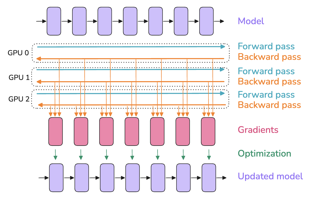 Figure 7: Data parallelism replicates the model N times across N devices. Each device processes a fraction of the batch and the resulting gradients are averaged across devices using an AllReduce operation. (Playbook, Section: Data Parallelism)
A simple implementation might perform the AllReduce operation only after the entire backward pass computation for $g_k$ is complete on all workers. This approach, however, leaves the communication network idle during computation and the compute units idle during communication. Performance can often be improved by overlapping communication and computation. As the backward pass proceeds from the final layers towards the initial layers, gradients for parameters in later layers become available earlier. The AllReduce operation for these gradients can be initiated while the backward pass continues computing gradients for parameters in earlier layers. This requires mechanisms, often provided by distributed training frameworks, to track gradient readiness and initiate communication asynchronously.
 Figure 8: Data Parallelism with Computation-Communication Overlap. Gradients (red boxes) for later layers can be communicated while gradients for earlier layers are still being computed. ("…gradients (red boxes) for a layer can be gathered and summed even before the gradients from earlier layers… have been computed… Overlapping computation and communication reduces the time spent waiting for gradient synchronization…" (Playbook, Section: Data Parallelism))
The primary communication cost in DP stems from the AllReduce operation performed on the gradients in each step. Backpropagation computes gradients sequentially, starting from the final layers of the model. A naive approach might wait until all gradients are computed before initiating a single large AllReduce operation. This minimizes the number of communication calls but prevents any overlap between gradient computation and communication. Alternatively, one could initiate a separate AllReduce for each gradient tensor immediately as it becomes available. However, this results in numerous small communication calls, incurring significant overhead from network latency and potentially underutilizing network bandwidth. Gradient bucketing offers a more efficient approach. Instead of communicating immediately, computed gradients $\nabla_w \ell(w, z)$ for various parameter blocks are grouped into larger, pre-defined buffers (“buckets”). An AllReduce operation is initiated only when a bucket is full. This strategy reduces the total number of communication calls compared to communicating each gradient individually, thus lowering latency overhead. It also allows for larger data transfers per call, potentially improving bandwidth utilization. Furthermore, while one bucket’s gradients are being communicated via AllReduce, the backward pass can continue computing gradients for subsequent layers and filling the next bucket, enabling overlap between computation and communication. The total time cost of the AllReduce depends on the number of model parameters $|w|$ (determining the total data volume) and the specific implementation details, including bucketing strategy and the communication bandwidth between workers.
 Figure 9: Data Parallelism with Gradient Bucketing. Gradients are grouped, and a single AllReduce is launched per bucket, enabling overlap. (Playbook, Section: Data Parallelism)
Gradient accumulation is often used with data parallelism to simulate larger effective batch sizes without increasing the instantaneous memory load per worker. Let the desired global batch size be $|\mathcal{B}|$, distributed across $N_d$ workers. Each worker $k$ is initially assigned a portion of the data $\mathcal{B}_k$, where $\cup_{k=1}^{N_d} \mathcal{B}_k = \mathcal{B}$ and $|\mathcal{B}_k| = |\mathcal{B}|/N_d$. To perform gradient accumulation over $A$ steps, each worker further divides its data portion $\mathcal{B}_k$ into $A$ smaller accumulation micro-batches $\mathcal{B}_{k,1}, \dots, \mathcal{B}_{k,A}$. For each accumulation step $a = 1, \dots, A$, worker $k$ performs a forward and backward pass using $\mathcal{B}_{k,a}$, computing the local gradient
\[g_{k,a} = \nabla_w \sum_{z \in \mathcal{B}_{k,a}} \ell(w, z).\]Instead of synchronizing immediately, worker $k$ accumulates these gradients locally, typically by summing them into a gradient buffer: $g_k^{(A)} = \sum_{a=1}^A g_{k,a}.$ Only after all $A$ accumulation steps are complete on all workers is the synchronization performed. The accumulated local gradients $g_k^{(A)}$ (which represent the gradient over the worker’s entire portion $\mathcal{B}_k$) are averaged across all $N_d$ workers using a single AllReduce operation to compute the final average gradient
\[\hat{g} = \frac{1}{N_d} \sum_{k=1}^{N_d} g_k^{(A)} = \frac{1}{|\mathcal{B}|} \sum_{k=1}^{N_d} \sum_{a=1}^A \sum_{z \in \mathcal{B}_{k,a}} \nabla_w \ell(w, z).\]A single optimizer step is then taken using this gradient $\hat{g}$. Crucially, gradient synchronization (AllReduce) must be disabled during the backward passes of the intermediate accumulation steps ($a=1, \dots, A-1$) and enabled only for the final step $A$. Frameworks often provide mechanisms, such as a no_sync() context manager in PyTorch’s DistributedDataParallel, to manage this synchronization correctly, avoiding unnecessary communication overhead.
Data parallelism effectively parallelizes computation across the data dimension by distributing batches over $N_d$ workers. This can significantly increase training throughput (samples processed per second). However, its primary limitation remains memory consumption. Every worker must store the entire set of model parameters $w$, the corresponding optimizer states (e.g., momentum $m_t$ and variance $v_t$ buffers for Adam, denoted $\text{OptState}$), the full gradients $g_k$ during accumulation or before synchronization, and the activations $A_{k,a}$ generated during the forward pass for its assigned micro-batch $\mathcal{B}_{k,a}$. Consequently, DP alone is insufficient if the model’s memory footprint (size of $w$ + size of $\text{OptState}$ + size of $A_{k,a}$ for a minimal batch) exceeds the memory capacity of a single worker. Furthermore, the performance of DP relies on efficient gradient synchronization. The communication cost of the AllReduce operation, which scales with the model size $|w|$ (number of parameters), can become a bottleneck, especially as the number of workers $N_d$ increases or if the interconnect bandwidth between workers is limited.
6.2 ZeRO (Zero Redundancy Optimizer) Stages
The ZeRO techniques address the memory limitations of standard Data Parallelism (DP) by eliminating redundant storage of model state across the $N_d$ workers in the DP group. Instead of each worker replicating the optimizer states (e.g., the momentum and second moment buffers for Adam; denoted by $\text{OptState}$), gradients ($g$), and potentially parameters ($w$), ZeRO partitions these states, assigning each worker $k$ responsibility for only a $1/N_d$ fraction of the total state. Let $w = \cup_{k=1}^{N_d} w^{(k)}$, $g = \cup_{k=1}^{N_d} g^{(k)}$, and $\text{OptState} = \cup_{k=1}^{N_d} \text{OptState}^{(k)}$ represent this conceptual partitioning, where worker $k$ owns shard $(k)$. (Playbook, Section: Zero Redundancy Optimizer)).
Activations $A_k$ depend on the local data $\mathcal{B}_k$ and cannot be sharded this way. However, optimizer states, gradients (after aggregation), and parameters are identical across replicas in standard DP and are thus candidates for partitioning. ZeRO implements this partitioning in three progressive stages.
ZeRO Stage 1 (ZeRO-1) partitions only the optimizer states. Each worker $k$ holds the full parameter set $w$ but only its shard of the optimizer state, $\text{OptState}^{(k)}$.
- Forward/Backward Pass: Each worker $k$ computes the full local gradient $g_k = \nabla_w \ell(w, \mathcal{B}_k)$.
- Gradient Synchronization/Sharding: A
ReduceScattercollective operation is used. It sums the gradients $g_k$ across all workers and distributes the result such that worker $k$ receives only the gradient shard $\hat{g}^{(k)}$ corresponding to the parameters $w^{(k)}$ whose optimizer states $\text{OptState}^{(k)}$ it owns. - Optimizer Step: Worker $k$ uses $\hat{g}^{(k)}$ and $\text{OptState}^{(k)}$ to update only its assigned parameter shard $w^{(k)}$ (often performing this update in higher precision, e.g., FP32).
- Parameter Synchronization: An
AllGathercollective is used to collect the updated parameter shards $w^{(k)}$ from all workers, reconstructing the complete, updated parameter set $w$ (typically in the working precision like BF16/FP16) on every worker for the next forward pass.
 Figure 10: ZeRO Stage 1 Communication Pattern. Optimizer states are sharded. Gradients are reduced and scattered, parameter updates happen locally, then parameters are gathered. (Playbook, Section: ZeRO-1: Partitioning Optimizer States)
ZeRO Stage 2 (ZeRO-2) partitions both optimizer states ($\text{OptState}^{(k)}$) and gradients. Worker $k$ still holds the full parameters $w$ temporarily during computation but only persists $\text{OptState}^{(k)}$ and its gradient shard $\hat{g}^{(k)}$.
- Forward Pass: Computes activations $A_k$.
- Backward Pass & Gradient Sharding: As gradients are computed, they are immediately reduced and scattered using
ReduceScatter. Worker $k$ only stores the final, averaged gradient shard $\hat{g}^{(k)}$ relevant to its optimizer states. This avoids storing the full gradient $g_k$ temporarily, saving memory compared to ZeRO-1. - Optimizer Step: Worker $k$ updates its parameter shard $w^{(k)}$ using $\hat{g}^{(k)}$ and $\text{OptState}^{(k)}$.
- Parameter Synchronization: An
AllGatherreconstructs the full parameters $w$ on all workers.
 Figure 11: ZeRO Stage 2 Communication Pattern. Adds gradient sharding to ZeRO-1. Gradients are reduced and scattered directly during the backward pass, avoiding temporary full gradient storage. Parameters are still gathered via AllGather after the optimizer step. (Playbook, Section: ZeRO-2: Adding Gradient Partitioning)
ZeRO Stage 3 (ZeRO-3 / FSDP) partitions all three components: parameters ($w^{(k)}$), gradients ($\hat{g}^{(k)}$), and optimizer states ($\text{OptState}^{(k)}$). Each worker $k$ persistently stores only its assigned shard $(k)$ of these states.
- Forward Pass: For each layer $j$ (or block of layers), workers perform an
AllGatheroperation to temporarily collect the necessary full parameter tensor(s) $W_j$ for that layer. They compute the forward pass for that layer, $A_j = f_j(A_{j-1}; W_j)$, and then immediately discard the parameter shards of $W_j$ they do not own. Only the output activations $A_j$ and the owned parameter shard $w^{(k)}_j$ are kept. - Backward Pass: Operates similarly. For layer $j$, the full parameters $W_j$ are gathered via
AllGather. The backward pass computes the gradient, but only the portion corresponding to the locally owned parameter shard, $\nabla_{w^{(k)}_j} \ell$, is stored. These local gradient pieces are then synchronized and averaged across workers usingReduceScatterto obtain the final gradient shard $\hat{g}^{(k)}_j$. - Optimizer Step: Worker $k$ updates its parameter shard $w^{(k)}$ using $\hat{g}^{(k)}$ and $\text{OptState}^{(k)}$. No final AllGather of parameters is needed, as they are gathered on-demand in the next forward pass.
 Figure 12: ZeRO-3 / FSDP Parameter Handling (Forward). Parameters are AllGathered before use and discarded afterward. Playbook, Section: ZeRO-3 Adding Parameter Partitioning
 Figure 13: ZeRO-3 / FSDP Parameter Handling (Backward). Similar to forward, parameters are gathered, used for gradient computation, and then gradients are ReduceScattered. Playbook, Section: ZeRO-3: Adding Parameter Partitioning
The progressive partitioning offered by ZeRO stages provides substantial memory savings for model state compared to standard DP. ZeRO-1 saves memory on optimizer states, ZeRO-2 adds savings on gradients, and ZeRO-3 provides the maximum savings by also partitioning the parameters themselves.
 Figure 14: ZeRO Memory Savings Overview. Illustrates theoretical memory reduction for parameters, gradients, and optimizer states per device for ZeRO stages 1, 2, and 3, compared to standard DP, as a function of DP group size N_d. Playbook, Section: ZeRO-3: Adding Parameter Partitioning
The primary advantage of ZeRO is enabling data parallel training for models far too large to fit in a single worker’s memory using standard DP. The main disadvantage is increased communication volume and complexity. ZeRO-1 and ZeRO-2 replace one gradient AllReduce with a ReduceScatter and add one parameter AllGather per step. ZeRO-3 replaces the single parameter AllGather with potentially many AllGather operations throughout the forward and backward passes (one per sharded parameter block being accessed). Efficient implementations rely on overlapping communication (prefetching parameters) with computation. Importantly, ZeRO partitions model state ($w, g, \text{OptState}$) but does not partition activation memory $A_k$.
6.3 Tensor Parallelism (TP)
Tensor Parallelism (TP) operates within individual layers, parallelizing the execution of large operations, most notably the matrix multiplications central to transformer MHA and FFN layers. It addresses cases where even a single layer’s parameters or intermediate activations are too large for one device, or where computation within a layer needs to be accelerated. TP partitions the tensors and computations across a group of $N_{tp}$ workers. (Playbook, Section: Tensor Parallelism).
Consider a linear layer computing $Y = f(XA)$ where $X \in \mathbb{R}^{b \times s \times h_{in}}$ is the input activation and $A \in \mathbb{R}^{h_{in} \times h_{out}}$ is the weight matrix ($f$ could be identity or include bias/activation). TP typically splits the weight matrix $A$ across the $N_{tp}$ workers:
-
Column Parallelism: Split $A$ column-wise: $A = [A_1 | A_2 | \dots | A_{N_{tp}}]$, where each shard $A_k \in \mathbb{R}^{h_{in} \times (h_{out}/N_{tp})}$. The input $X$ must be fully available to all $N_{tp}$ workers. Each worker $k$ computes a corresponding shard of the output: $Y_k = f(X A_k) \in \mathbb{R}^{b \times s \times (h_{out}/N_{tp})}$. The full output $Y$ is represented by the concatenation $Y = [Y_1 | \dots | Y_{N_{tp}}]$ across the workers’ memory. In the backward pass, computing the gradient w.r.t. $X$ involves summing contributions from all workers: $\nabla_X \ell = \sum_{k=1}^{N_{tp}} (\nabla_{Y_k} \ell) A_k^T$, typically requiring an
AllReduceoperation. -
Row Parallelism: Split $A$ row-wise: $A = [A_1^T | \dots | A_{N_{tp}}^T]^T$, where $A_k \in \mathbb{R}^{(h_{in}/N_{tp}) \times h_{out}}$. The input $X$ must also be sharded column-wise (along the $h_{in}$ dimension): $X = [X_1 | \dots | X_{N_{tp}}]$, where $X_k \in \mathbb{R}^{b \times s \times (h_{in}/N_{tp})}$. This sharding often naturally results from a preceding column-parallel layer. Each worker $k$ computes a partial output using its input and weight shards: $Y_k = f(X_k A_k)$. The final output $Y \in \mathbb{R}^{b \times s \times h_{out}}$ is obtained by summing these partial outputs across all workers: $Y = \sum_{k=1}^{N_{tp}} Y_k$, which requires an
AllReduceoperation. In the backward pass, the gradient $\nabla_Y \ell$ flowing from subsequent computations is available on all workers; each worker $k$ then computes the gradient with respect to its input shard locally using the formula $\nabla_{X_k} \ell = (\nabla_Y \ell) A_k^T$ and its local weight shard $A_k$.
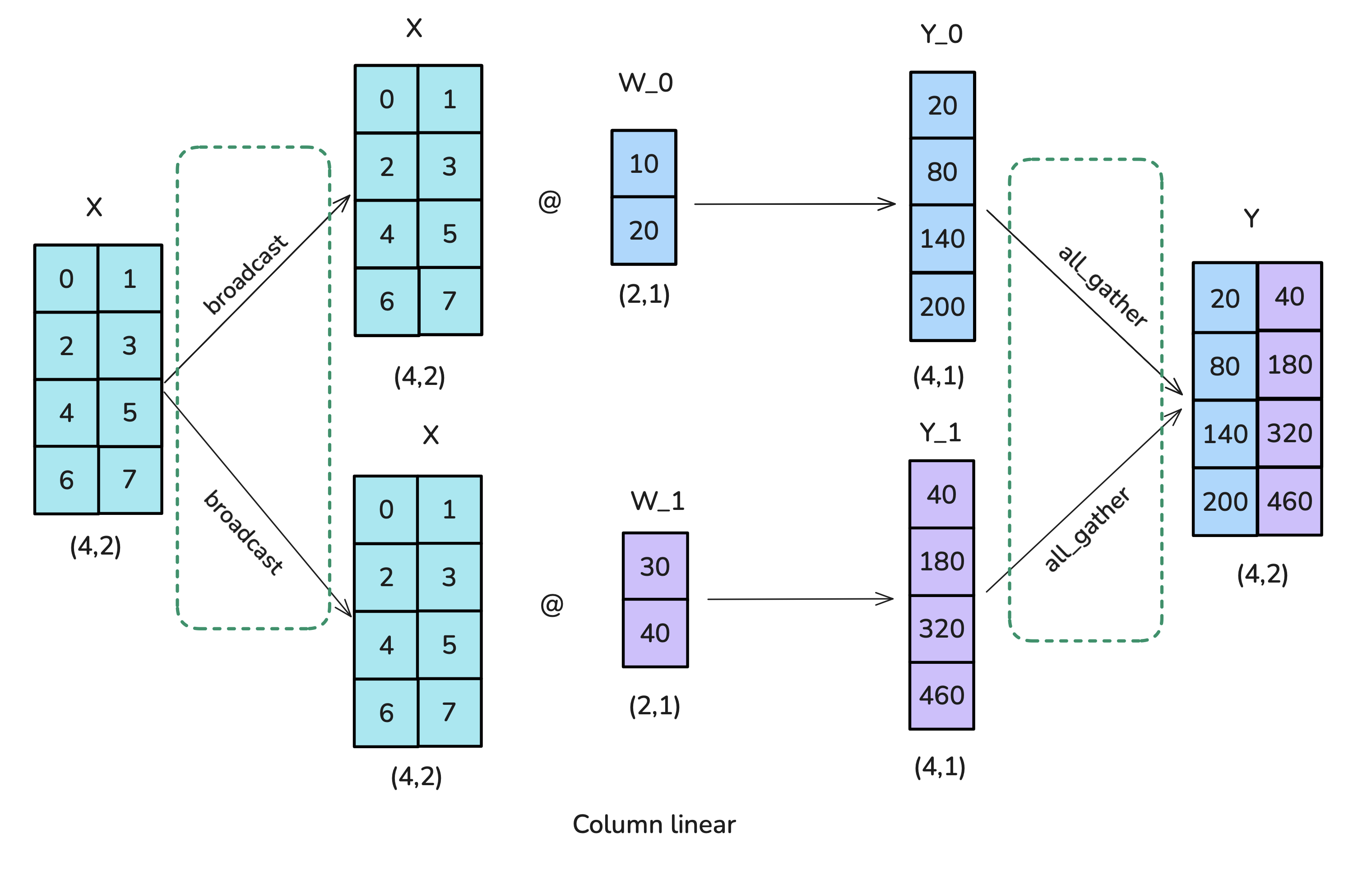 Figure 15: Tensor Parallelism for Linear Layers (Column). Playbook, Section: Tensor Parallelism
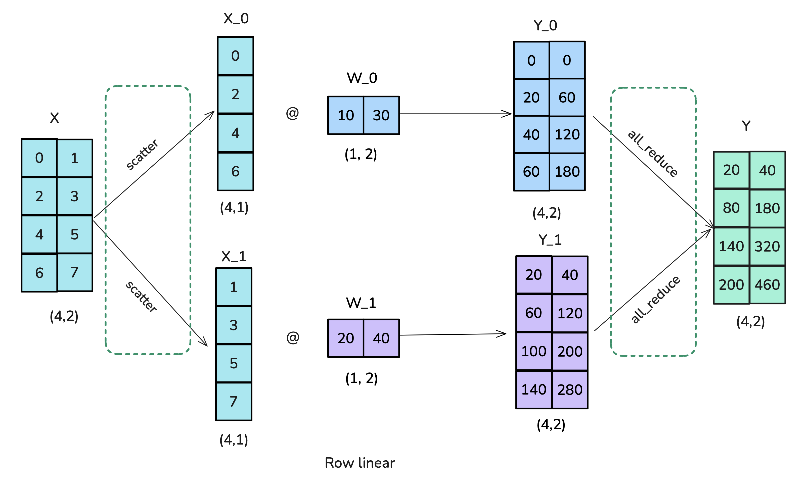 Figure 16: Tensor Parallelism for Linear Layers (Row). Playbook, Section: Tensor Parallelism
In transformer blocks, FFN layers are commonly parallelized using column parallelism for the first linear layer ($W_1$) followed by row parallelism for the second ($W_2$). This pattern, sometimes called MLP parallelism, avoids an AllReduce between the two layers. MHA layers use column parallelism for the $Q, K, V$ projections ($W_Q, W_K, W_V$) and row parallelism for the output projection ($W_O$).
More specifically, specific tensor parallelism strategies are applied to the FFN and MHA layers to optimize communication.
For FFN layers (often structured as $Y = f(XW_1)W_2$ where $f$ is an activation like GELU):
- The first linear layer ($W_1 \in \mathbb{R}^{h \times d_{ff}}$) uses column parallelism. Input $X \in \mathbb{R}^{b \times s \times h}$ (assumed available to all workers) is multiplied by the column-sharded weight $W_{1,k} \in \mathbb{R}^{h \times (d_{ff}/N_{tp})}$. Each worker $k$ computes $Z_k = X W_{1,k}$. The activation $f$ is applied element-wise, resulting in $f(Z_k)$. The intermediate tensor $f(Z)$ is now effectively sharded along the intermediate dimension ($d_{ff}$).
- The second linear layer ($W_2 \in \mathbb{R}^{d_{ff} \times h}$) uses row parallelism. The weight $W_2$ is split row-wise ($W_{2,k} \in \mathbb{R}^{(d_{ff}/N_{tp}) \times h}$), matching the sharding dimension of the input $f(Z)=[f(Z_k)]$. Each worker $k$ computes a partial output $Y_k = f(Z_k) W_{2,k}$.
- Crucially, no communication is needed between the two linear layers because the output sharding of the first layer aligns perfectly with the input sharding required by the second layer.
- The final output $Y$ is obtained by summing the partial outputs across workers: $Y = \sum_{k=1}^{N_{tp}} Y_k$, requiring a single
AllReduceoperation at the end of the FFN block. This combined column-then-row pattern is sometimes called MLP parallelism.
For MHA layers:
- The Q, K, and V projection layers ($W_Q, W_K, W_V \in \mathbb{R}^{h \times h}$) use column parallelism. Input $X$ is multiplied by column-sharded weights $W_{Q,k}, W_{K,k}, W_{V,k}$ (producing Q1/K1/V1 and Q2/K2/V2 in Figure 17) to produce $Q_k, K_k, V_k$. This effectively shards the Q, K, V tensors (and the attention heads) along the hidden dimension $h$ across the $N_{tp}$ workers.
- Attention Computation (Head-Wise Parallelism): As shown in Figure 16, if the TP degree $N_{tp}$ divides the number of attention heads $a$, the attention computation can be performed entirely locally on each worker $k$. Each worker calculates attention only for its subset of heads using its local shards $Q_k, K_k, V_k$ (i.e., $\text{softmax}(Q_k K_k^T / \sqrt{d_k}) V_k$). This efficient head-wise sharding avoids the need for an internal
AllGatherof K and V tensors that would be required in more general TP splits of attention. The output $Attn = [Y_1, Y_2, \dots]$ remains sharded along the hidden dimension. - The final output projection layer ($W_O \in \mathbb{R}^{h \times h}$, represented as B1/B2 in Figure 17) uses row parallelism. The weight $W_O$ is split row-wise ($W_{O,k} \in \mathbb{R}^{(h/N_{tp}) \times h}$), matching the sharding of the input $Attn=[Y_k]$. Each worker $k$ computes a partial output $Z_k = Attn_k W_{O,k}$ (shown as Y1 B1 -> Z1 and Y2 B2 -> Z2).
- Similar to the FFN, the final MHA output $Y$ is obtained by summing the partial outputs: $Y = \sum_{k=1}^{N_{tp}} Z_k$, requiring an
AllReduceoperation (explicitly shown combining Z1 and Z2 in Figure 17).
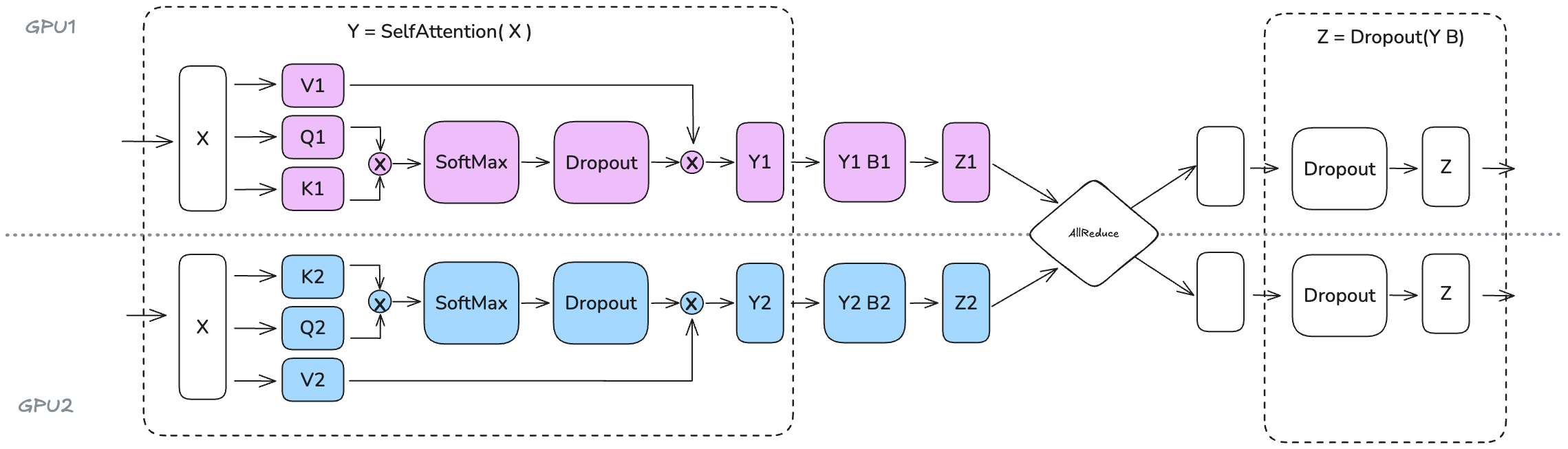 Figure 17: Tensor Parallelism Applied to Transformer Blocks (TP=2). This illustrates the common head-wise parallelism for attention, where Q/K/V projections use column parallelism, attention calculation is local per GPU for its assigned heads (avoiding internal AllGather), and the output projection uses row parallelism followed by an AllReduce. The FFN follows a column-parallel then row-parallel pattern, also requiring a final AllReduce. (Playbook, Section: Tensor Parallelism)
For MHA, this efficient head-wise parallel computation requires the number of attention heads $a$ to be divisible by the TP degree $N_{tp}$.
TP requires collective communication operations (like AllReduce) within the forward and backward computations of individual layers. This implies frequent synchronization and necessitates very high-bandwidth, low-latency interconnects between the participating workers, such as NVLink typically found within a single compute node.
 Figure 18: Communication Timeline in Tensor Parallelism. ("…we hit a synchronization point with the AllReduce operation that cannot be overlapped with computation. This exposed communication overhead is necessary to combine partial results across tensor-parallel ranks…" (Playbook, Section: Tensor Parallelism)
The main benefit of TP is reducing the memory footprint per worker for weights $w$, gradients $g$, optimizer states $\text{OptState}$, and activations $A$ associated with the parallelized layers, as these are sharded across the $N_{tp}$ workers. This allows fitting larger layers onto devices. TP can also reduce the wall-clock time per layer if computation savings dominate the added communication cost. However, the high communication overhead limits TP’s scalability, making it most effective across a small number of tightly connected workers (e.g., $N_{tp} \le 8$). It also increases implementation complexity significantly. Furthermore, operations that require the full hidden dimension (like Layer Normalization) cannot be directly parallelized by TP along the hidden dimension, limiting overall activation memory savings unless combined with other techniques like Sequence Parallelism.
6.4 Sequence Parallelism (SP)
Sequence Parallelism (SP) is an optimization technique used in conjunction with Tensor Parallelism (TP) to further reduce activation memory. TP effectively shards tensors along the hidden dimension ($h$) for matrix multiplications but struggles with operations like Layer Normalization or Dropout that typically require the full activation vector for each token. SP addresses this by sharding activations along the sequence dimension ($s$) specifically for these non-TP-friendly operations, while using TP’s hidden dimension sharding for the matrix multiplies. (Playbook, Section: Sequence Parallelism).
This necessitates transitions between sequence-sharded and hidden-sharded tensor representations. Consider the data flow illustrated in Figure 18, using TP degree $N_{tp}=2$:
- SP Region (e.g., LayerNorm): Input activations $X$ arrive sharded along the sequence dimension (worker $k$ holds $X_k \in \mathbb{R}^{b \times (s/N_{tp}) \times h}$). LayerNorm is applied locally by each worker to its chunk.
- Transition SP -> TP (
g): Before a column-parallel TP operation (like the first linear layer $A_1$, $W_1$), which requires input sharded along the hidden dimension $h$ but complete along $s$, an AllGather collective (g) is performed along the sequence dimension. This reconstructs the full activation tensor $Y \in \mathbb{R}^{b \times s \times h}$ on each TP worker. - TP Region (e.g., FFN): The column-parallel linear layer $A_1$ processes $Y$, outputting activations $Z$ sharded along the intermediate hidden dimension. After the activation function (e.g., GELU), the row-parallel linear layer $B_1$ ($W_2$) takes this hidden-sharded input and produces partial output tensors $W_k$.
- Transition TP -> SP (
g*): To transition back to sequence-sharding for a subsequent SP-region operation (like Dropout), a ReduceScatter collective (g*) is used. This operation efficiently performs two tasks simultaneously: (i) it sums (reduces) the partial outputs $W_k$ across TP ranks, completing the row-parallel computation, and (ii) it scatters the final summed result, partitioning it along the sequence dimension $s$. The output $W^* $ is now correctly sharded as $W_k^* \in \mathbb{R}^{b \times (s/N_{tp}) \times h}$. - SP Region (e.g., Dropout): Dropout is applied locally by each worker to its sequence-sharded chunk $W_k^*$.
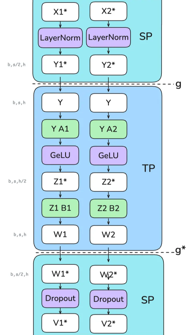 Figure 19: Tensor Sharding and Communication Transitions for Sequence Parallelism (SP) combined with Tensor Parallelism (TP). The diagram shows activations starting sharded along the sequence dimension (
s) for LayerNorm (SP region). An AllGather (g) along s prepares the full tensor for the TP region (Column-Linear A1, GELU, Row-Linear B1), where activations are sharded along the hidden dimension (h). A ReduceScatter (g*) performs the necessary summation for the row-parallel layer B1 while simultaneously scattering the result along s for the subsequent Dropout (SP region). (Playbook, Section: Sequence Parallelism)
The overall communication volume with SP is generally similar to TP alone, but the collectives change from AllReduce to combinations of AllGather and ReduceScatter along the sequence dimension, still demanding high-bandwidth interconnects.
The primary benefit of Sequence Parallelism is reducing peak activation memory by avoiding materialization of the full $b \times s \times h$ tensor during operations like LayerNorm or Dropout. This allows for larger batch sizes or longer sequences within a TP group but adds complexity due to the sharding transitions.
6.5 Context Parallelism (CP) & Ring Attention
While Tensor Parallelism (TP) combined with Sequence Parallelism (SP) helps manage activation memory, extremely long input sequences ($s$) can still lead to prohibitive activation memory usage, especially during attention computation which scales quadratically with $s$. Context Parallelism (CP) is a technique designed for such scenarios. It partitions the input sequence globally across a group of $N_{cp}$ workers for most computations. Each worker $k$ is assigned a distinct chunk of the sequence $X_k \in \mathbb{R}^{b \times (s/N_{cp}) \times h}$. (Playbook, Section: Context Parallelism).
Standard Transformer operations like Feedforward Networks (FFN) and Layer Normalization operate independently on each token representation. Under CP, these can be performed locally on each worker’s sequence chunk $X_k$ without requiring communication between CP ranks.
The primary communication challenge arises within the self-attention mechanism. To compute the attention output for its local queries $Q_k$, worker $k$ requires access to the key ($K$) and value ($V$) representations corresponding to all tokens in the original sequence, including those residing on other workers. This necessitates an efficient inter-worker communication strategy for K/V tensors.
Ring Attention provides such a pattern. Workers are organized in a logical ring topology. The global attention computation proceeds over $N_{cp}-1$ communication steps. In each step $i$:
- Worker $k$ initiates a non-blocking send of its current key/value chunk ($K_{curr}, V_{curr}$) to the next worker in the ring, $(k+1) \pmod{N_{cp}}$.
- Worker $k$ computes the partial attention output using its local queries $Q_k$ and the locally available chunk ($K_{curr}, V_{curr}$). This overlaps computation with the ongoing communication.
- Worker $k$ performs a blocking receive for the key/value chunk ($K_{prev}, V_{prev}$) sent by the previous worker, $(k-1) \pmod{N_{cp}}$. This received chunk becomes the ($K_{curr}, V_{curr}$) for the subsequent step ($i+1$).
This structured exchange allows the point-to-point communication of K/V chunks to be largely hidden by the local attention computations.
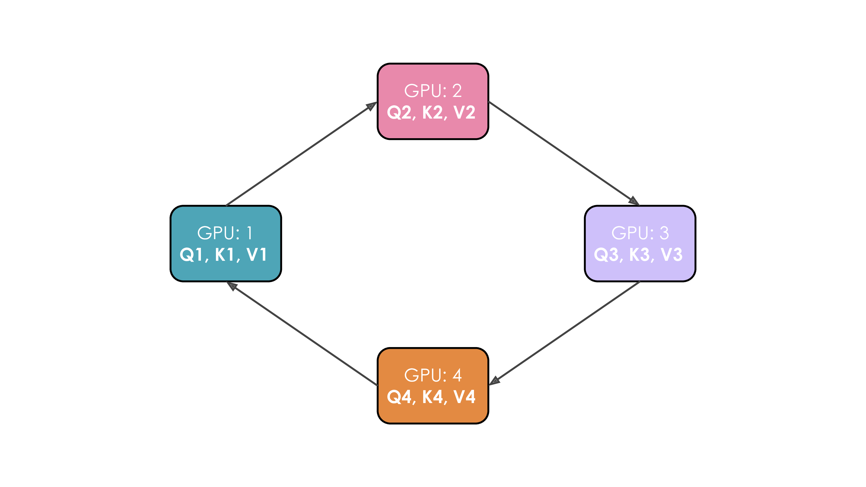 Figure 20: Ring Attention Mechanism. Illustrates the step-by-step passing of K/V chunks around a ring of 4 GPUs. Asynchronous sends (step 1) and local computation (step 2) overlap with waiting for receives (step 3) from the neighboring worker. (“each GPU first initiates an asynchronous communication… computes the attention score… receives keys and values from the previous GPU…” (Playbook, Section: Context Parallelism))
A specific challenge occurs when applying CP to models using causal attention masks, where a token $i$ only attends to tokens $j \le i$. If the sequence is partitioned sequentially across workers (GPU 0 gets first chunk, GPU 1 gets second, etc.), the causal mask results in significantly less computational work (fewer $QK^T$ dot products) for workers holding earlier sequence chunks compared to those holding later chunks. This creates a substantial load imbalance, as depicted in Figure 20.
 Figure 21: Attention Computation Load with Naive Sequential Partitioning and Causal Mask (16 tokens, 4 GPUs). Colors map tokens to GPUs (GPU1=teal, GPU2=pink, GPU3=purple, GPU4=orange). Shaded cells indicate necessary $QK^T$ calculations. GPU 1 performs far fewer calculations than GPU 4, illustrating load imbalance. (Playbook, Section: Context Parallelism)
ZigZag attention partitioning resolves this load imbalance. It distributes sequence chunks non-contiguously among workers, ensuring each worker processes a mixture of early and late sequence positions. This method balances the computational load imposed by the causal mask across all workers in the CP group, as shown in Figure 21.
 Figure 22: ZigZag Partitioning for Load Balancing in Causal Ring Attention. Non-contiguous chunk assignment (indicated by colors matching Figure 21) distributes the computational load (shaded cells) more evenly across the 4 GPUs when a causal mask is applied. (“…assigning the tokens not purely sequential to the GPUs but by mixing the ordering… computation is now balanced across all GPUs.” (Playbook, Section: Context Parallelism))
In summary, the communication requirements for Context Parallelism are:
- Point-to-point communication (typically using the Ring Attention pattern) for K/V chunk exchange within the attention mechanism.
- An
AllReduceoperation across the $N_{cp}$ group after the full backward pass to average gradients, necessary because each worker computes gradients based on different input data (sequence chunks).
Context Parallelism, utilizing Ring Attention, enables training on very long sequences by maintaining sequence-sharded activations for most layers. However, it introduces implementation complexity within the attention mechanism and necessitates gradient synchronization across the CP group.
6.6 Pipeline Parallelism (PP) & Scheduling
Pipeline Parallelism (PP) is primarily employed when the model parameters $|w|$ are too large to fit onto a single device or even a Tensor Parallelism group, or when scaling training across a large number of compute nodes where TP’s high intra-node bandwidth assumption does not hold. PP partitions the model layers sequentially into $P$ stages. Each stage $p \in {1, \dots, P}$, consisting of a contiguous block of layers with parameters $w_p$, is assigned to a different worker or group of workers (forming a pipeline group of size $N_p = P$). Data flows sequentially through the pipeline: the output activations $A_p$ of stage $p$ become the input $A_{p}$ for stage $p+1$. Formally, $A_p = f_p(A_{p-1}; w_p)$, where $f_p$ represents the computation of stage $p$. (Playbook, Section: Pipeline Parallelism).
Executing this sequentially for a full data batch $\mathcal{B}$ (i.e., computing $A_1 = f_1(\mathcal{B})$, then $A_2 = f_2(A_1)$, …, then performing the full backward pass) is highly inefficient. At any moment, only one stage $p$ is active (either computing $f_p$ or its backward counterpart $b_p$), leaving the other $P-1$ stages idle. This idle time is referred to as the “pipeline bubble.” The fraction of idle time increases with the number of stages $P$, significantly hindering hardware utilization.
 Figure 23: Pipeline Bubble in Naive Sequential Execution. ("An example of Pipeline parallelism… The remaining idle time is indicated in grey and usually called the ‘bubble’…" (Playbook, Section: Pipeline Parallelism))
To reduce the pipeline bubble, the global data batch $\mathcal{B}$ is split into $m$ smaller micro-batches, $\mathcal{B}^{(1)}, \dots, \mathcal{B}^{(m)}$. The pipeline processes these micro-batches in a staggered fashion, allowing different stages to work on different micro-batches concurrently. The specific order of forward ($F$) and backward ($B$) passes for micro-batches defines the pipeline schedule. Common schedules include:
-
All-Forward-All-Backward (AFAB) / GPipe: All micro-batches complete their forward pass through all $P$ stages ($F_1^{(j)}, F_2^{(j)}, \dots, F_P^{(j)}$ for $j=1..m$). Only then does the backward pass begin for all micro-batches ($B_P^{(j)}, B_{P-1}^{(j)}, \dots, B_1^{(j)}$ for $j=1..m$). This schedule is relatively simple but requires storing the activations $A_{p-1}^{(j)}$ for all micro-batches $j$ at each stage boundary $p$ until the corresponding backward pass $B_p^{(j)}$ is executed. Peak activation memory is roughly proportional to $m$. The relative size of the bubble (fraction of idle time) is reduced to approximately $(P-1)/m$.
-
One-Forward-One-Backward (1F1B) / Interleaved: This schedule interleaves forward and backward passes more tightly to reduce activation memory. For example, after micro-batch $j$ completes its forward pass $F_P^{(j)}$, its backward pass $B_P^{(j)}, \dots, B_1^{(j)}$ can begin immediately, potentially overlapping with the forward passes $F_1^{(j+k)}, \dots, F_P^{(j+k)}$ of subsequent micro-batches. This significantly reduces the number of activations that need to be stored simultaneously, with peak activation memory roughly proportional to the number of stages $P$ rather than the number of micro-batches $m$. The bubble size remains approximately $(P-1)/m$, but implementation complexity increases.
 Figure 24: Pipeline Schedule: All-Forward-All-Backward (GPipe-like). ("GPipe (All Forward All Backward)… stores the activations for all micro-batches" (Playbook, Section: Pipeline Parallelism))
 Figure 25: Pipeline Schedule: One-Forward-One-Backward (Interleaved). ("1F1B… reduces the memory footprint… by performing backward passes as soon as possible" (Playbook, Section: Pipeline Parallelism))
More advanced schedules aim to further reduce or eliminate the bubble. Interleaved Stages (not the same as 1F1B scheduling) assign non-contiguous layers to pipeline stages (e.g., layers 1,3,5 on stage 1; layers 2,4,6 on stage 2) which can sometimes reduce dependencies and bubble size but increases inter-stage communication. Techniques like ZeroBubble or DualPipe use fine-grained analysis of backward pass dependencies (separating weight gradient calculation $\nabla w_p$ from input gradient calculation $\nabla A_{p-1}$) to construct complex schedules that achieve near-zero bubble size, often at the cost of significantly increased implementation difficulty.
Communication in PP mainly involves point-to-point transfers of activation tensors $A_p^{(j)}$ forward and gradient tensors $\nabla A_p^{(j)}$ backward between adjacent pipeline stages ($p$ and $p+1$). The size of these transfers depends on the batch size, sequence length, hidden dimension, and the micro-batch size $m$. This communication pattern is generally less demanding on network bandwidth compared to the large collective operations in TP or FSDP, making PP suitable for scaling across multiple compute nodes with standard network interconnects.
Pipeline Parallelism excels at partitioning very deep models across many devices, enabling the training of models whose total parameter count $|w|$ is extremely large. It is generally less sensitive to inter-node communication bandwidth than TP or FSDP. However, the pipeline bubble inherently limits perfect scaling efficiency. Achieving good performance requires careful load balancing (ensuring each stage $p$ has similar computational cost) and selecting an appropriate schedule (trading off activation memory, bubble size, and complexity).
6.7 Expert Parallelism (EP)
Expert Parallelism (EP) is a specialized technique applicable only to Mixture-of-Experts (MoE) models. MoE architectures modify standard transformer blocks by replacing certain layers, typically the FFN, with a collection of $E$ parallel “expert” networks (usually FFNs themselves), ${f_{expert, e}}_{e=1}^E$. For each input token representation $x_t$, a lightweight gating network $R(x_t)$ dynamically selects a small subset of these experts (often just the top 1 or top 2) to process that specific token. (Playbook, Section: Expert Parallelism).
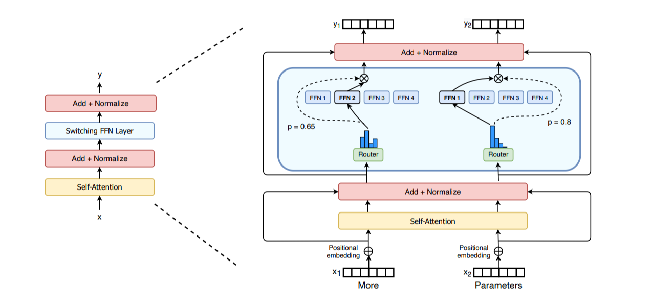 Figure 26: Mixture-of-Experts (MoE) Layer Concept. Source: Switch Transformers: Scaling to Trillion Parameter Models with Simple and Efficient Sparsity
(Fedus, W et al. (2022)) paper Playbook, Section: Expert Parallelism
Figure 26: Mixture-of-Experts (MoE) Layer Concept. Source: Switch Transformers: Scaling to Trillion Parameter Models with Simple and Efficient Sparsity
(Fedus, W et al. (2022)) paper Playbook, Section: Expert Parallelism
Expert Parallelism distributes these $E$ expert networks across a group of $N_{ep}$ workers. Worker $k$ might hold the parameters $w_e$ for a subset of experts $E_k$. Since only a few experts process each token, EP leverages this sparsity. During the forward pass, after the gating network $R$ determines the expert assignment $e(x_t)$ for each token representation $x_t$, an AlltoAll collective communication operation is performed. This operation efficiently routes each token $x_t$ from its current worker to the specific worker(s) responsible for holding the assigned expert(s) $e(x_t)$. The receiving worker $k$ then computes the expert output $y_t = f_{expert, e(x_t)}(x_t; w_{e(x_t)})$. A second AlltoAll operation is used to gather the computed outputs $y_t$ back to their original workers, combining them according to the gating weights. A similar pattern occurs in the backward pass.
Expert Parallelism by itself only parallelizes the MoE layers. Other model components (like attention layers or non-MoE FFNs) would still be replicated and perform redundant computations across the $N_{ep}$ workers. Therefore, EP is almost always used in combination with Data Parallelism (DP). The workers are arranged conceptually in a 2D grid of size $N_d \times N_{ep}$. Within each row (fixed DP rank), workers perform EP, distributing the experts. Within each column (fixed EP rank), workers perform DP, replicating the non-expert parts of the model and the expert parameters assigned to that column, while processing different slices of the data batch. Gradient synchronization for the non-expert parameters occurs via AllReduce within each EP group (column), while token routing for experts occurs via AlltoAll within each DP group (row).
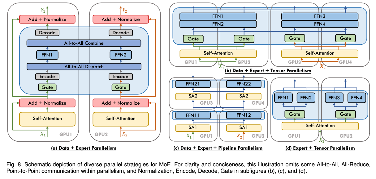 Figure 27: Combining Expert Parallelism (EP) and Data Parallelism (DP). Source: A Survey on Mixture-of-Experts Models (Cai, Z., et al. (2024). (Playbook, Section: Expert Parallelism)
Expert Parallelism enables scaling models to extremely large parameter counts (by increasing the number of experts $E$) while keeping the computational cost (FLOPs) per token relatively low, as each token only passes through a small number of experts. The main challenge is the communication overhead associated with the AlltoAll operations required for routing tokens, which can be significant, especially as the number of experts and workers increases. EP is inherently tied to the MoE architecture.
7. Combining Strategies & Conclusion
The parallelism strategies discussed in Section 6—Data Parallelism (DP/ZeRO), Pipeline Parallelism (PP), Tensor Parallelism (TP/SP/CP), and Expert Parallelism (EP)—each address specific bottlenecks in large-scale training. However, each also has limitations. Standard DP is constrained by single-device memory; ZeRO increases communication volume; TP scalability is typically limited by intra-node bandwidth; PP introduces pipeline bubbles; CP adds overhead for long sequences; EP applies only to MoE models. Consequently, training the largest state-of-the-art models almost always requires combining multiple parallelism strategies to leverage their complementary strengths while mitigating their individual weaknesses (Playbook, Section: 5D Parallelism in a Nutshell).
A common and foundational approach is 3D Parallelism, which combines Data Parallelism ($N_d$ workers), Pipeline Parallelism ($P$ stages), and Tensor Parallelism ($N_{tp}$ workers). The total number of workers is $N = N_d \times P \times N_{tp}$. Conceptually, these workers are arranged in a 3D grid. The typical mapping leverages hardware topology: TP is used within a compute node, utilizing high-speed interconnects like NVLink among its $N_{tp}$ workers to handle the frequent communication required for intra-layer parallelism. PP is used across nodes, partitioning the model’s layers sequentially into $P$ stages, relying on the less frequent inter-stage communication (activations forward, gradients backward) which can tolerate slower inter-node network bandwidth. DP then replicates this entire PP+TP structure $N_d$ times, processing different data batches on each replica, with gradient synchronization occurring across these replicas.
In modern large-scale training, the Data Parallelism dimension ($N_d$) within combined strategies like 3D parallelism is often implemented using ZeRO, particularly ZeRO-3/FSDP, rather than standard DP. The primary benefit is memory efficiency. By sharding the model parameters $w$, gradients $g$, and optimizer states $\text{OptState}$ across the $N_d$ workers (Section 6.2), FSDP drastically reduces the memory required per worker compared to replicating the full model state. This allows the combined system (e.g., FSDP + PP + TP) to accommodate significantly larger models or use larger per-replica batch sizes than would be possible with standard DP + PP + TP. While simpler ZeRO stages like ZeRO-1 or ZeRO-2 can also be combined with PP to save optimizer state or gradient memory respectively, FSDP offers the most substantial savings by partitioning the parameters themselves.
When considering how to partition large model parameters across devices, Pipeline Parallelism (PP) and ZeRO-3 (FSDP) offer different approaches, as highlighted in the playbook (Playbook, Section: 5D Parallelism in a Nutshell). PP partitions the model layer-wise into sequential stages; worker $p$ holds the full parameters $w_p$ for the layers in its stage. ZeRO-3 partitions parameter-wise across DP workers; worker $k$ holds shards $w^{(k)}$ of parameters from all layers. This leads to different communication patterns: PP primarily communicates activations $A_p$ and activation gradients $\nabla A_p$ between stages via point-to-point messages, whereas ZeRO-3 communicates parameter shards $w^{(k)}$ via AllGather collectives within the forward/backward pass. Consequently, their performance sensitivities differ: PP’s efficiency is heavily influenced by the pipeline bubble, which can be mitigated by increasing the number of micro-batches (often related to gradient accumulation grad_acc); ZeRO-3’s efficiency relies on overlapping the parameter AllGather communication with computation, which typically benefits from larger micro-batch sizes (mbs) or sequence lengths (s). While combining PP and ZeRO-3 is technically possible, the playbook notes it can be complex and may demand very large global batch sizes to amortize the communication overheads effectively.
Context Parallelism (CP) and Expert Parallelism (EP) are typically viewed as orthogonal additions, layered onto a base parallelism configuration (like FSDP + PP + TP) to address specific needs. CP is employed when dealing with extremely long sequences ($s$), adding sequence-dimension sharding and Ring Attention communication, usually across the DP or PP dimension workers. EP is used exclusively for MoE models, distributing the expert networks across a dimension of workers (often the DP dimension) and introducing AlltoAll communication for token routing.
The interplay between these strategies allows for flexible configurations tailored to specific model sizes and hardware capabilities. The following diagram and table summarize the core ideas and trade-offs.
 Figure 26: Conceptual Overview of Combined Parallelism Dimensions. Playbook, Section: 5d_parallelism_in_a_nutshell
Table 1: Summary of Parallelism Strategies

Choosing the optimal combination and configuration involves a structured process, as outlined in the playbook (Playbook, Section: Finding the Best Training Configuration). The general approach involves iterative refinement: first, ensuring a single training step fits in memory using necessary parameter partitioning (PP, TP, ZeRO-3) and activation management (recomputation); second, scaling to the target global batch size using data-centric parallelism (DP/FSDP, CP) and gradient accumulation; and third, optimizing for throughput by tuning the degrees of parallelism (e.g., maximizing intra-node TP) and micro-batch sizes while respecting communication bottlenecks. The best strategy is highly dependent on the specific model architecture, the number and type of available accelerators, and the characteristics of the network interconnects.
In conclusion, training large-scale transformer models pushes the boundaries of computation and memory available on single devices. Addressing this requires moving beyond individual optimizers to system-level parallelism strategies. We have reviewed the transformer architecture’s demands, the critical bottleneck of activation memory, and the utility of activation recomputation. We explored the primary parallelism techniques detailed in the Ultrascale Playbook: Data Parallelism (enhanced by ZeRO/FSDP), Pipeline Parallelism, Tensor Parallelism (enhanced by SP), Context Parallelism, and Expert Parallelism. Successful training at the largest scales necessitates thoughtfully combining these techniques—often in a 3D (DP/FSDP + PP + TP) or more complex arrangement—to optimally balance computation, memory usage, and communication overhead for the specific model and hardware infrastructure. Resources like the Ultrascale Playbook provide invaluable practical guidance for navigating these complex trade-offs.