Stat 4830 Recap: Optimization in PyTorch - Cheat Sheet

Overall Goal: Consolidate understanding of numerical optimization for ML/Data Science using PyTorch, aiming to become an intelligent consumer of these methods.

---

1. Introduction

• Purpose: Final recap of Stat 4830. Consolidate concepts and skills.
• Course Theme: Formulating & solving numerical optimization problems for ML/Data Science. Emphasis on practical PyTorch implementation.
• Project Role: Provided hands-on application experience.
• Syllabus Goal: “Become an intelligent consumer of numerical methods and software for solving modern optimization problems.” This recap reinforces that goal.

---

2. Key Concepts & Skills

PyTorch Fundamentals

• Started with basics: Tensors, Linear Algebra (Lecture 1).
• Core Concept: Automatic Differentiation (autograd) (Lecture 4).
• Calculus View: Derivative/Jacobian = Best Linear Approximation; autograd implements chain rule (Lecture 5).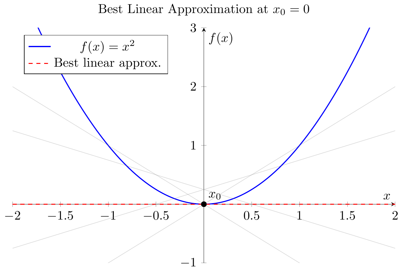
  • Figure 2.1: Derivative as best linear approx. Tangent line gives closest linear fit near a point. (Lecture 5)
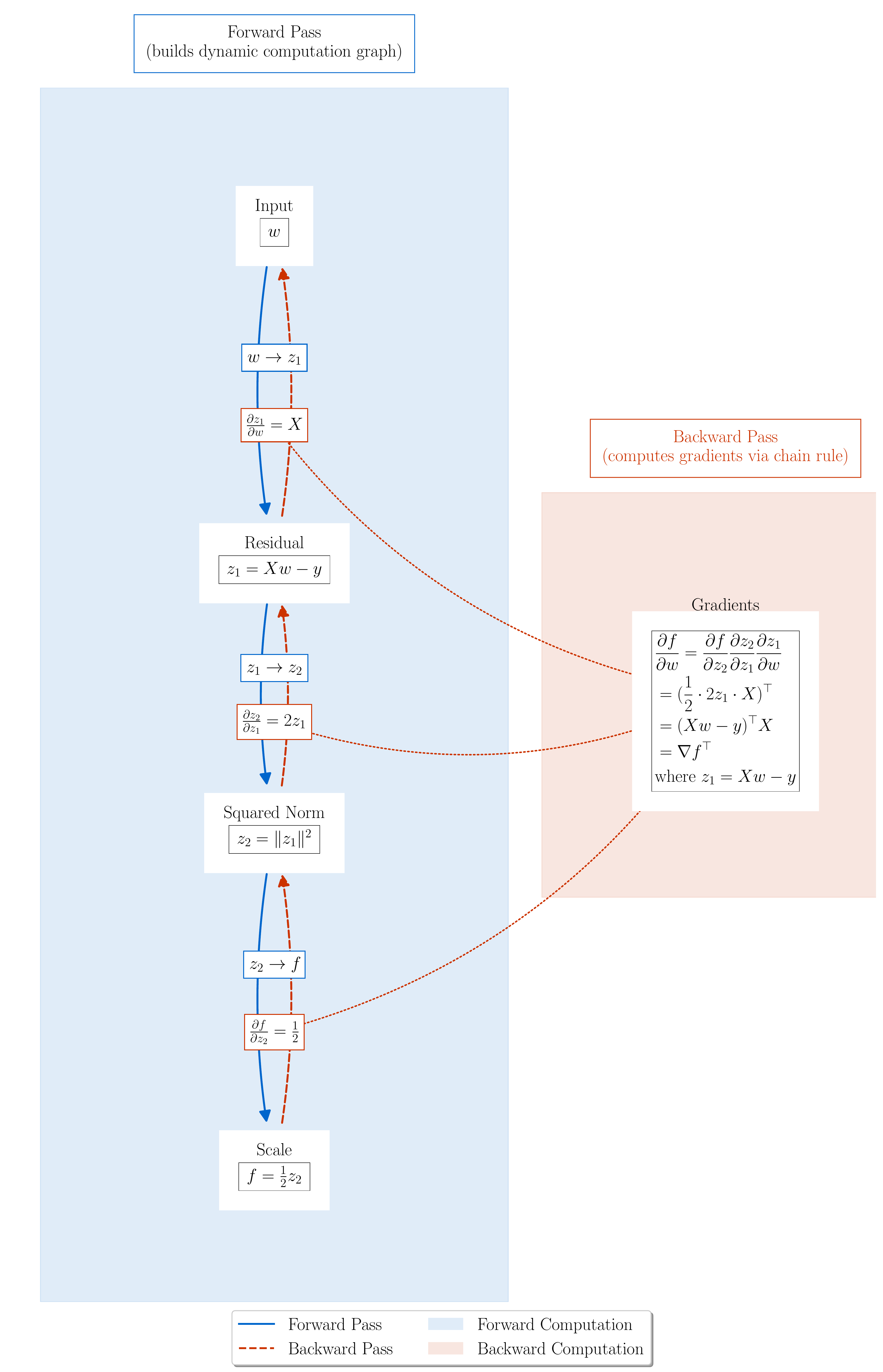
  • Figure 2.2: Computational graph for Least Squares loss $L(w) = \frac{1}{2}|Xw - y|^2$. autograd builds this graph during the forward pass and uses it to compute gradients via the chain rule during backward(). (Lecture 4)
• Key Tools: nn.Module (models), DataLoader (data), torch.optim (optimizers), torch.optim.lr_scheduler (schedules) (Lecture 8).

Problem Formulation

• Goal: Minimize objective $L(w)$, typically average loss $L(w) = \frac{1}{n}\sum_{i=1}^n \ell(w, z_i)$.
• Examples:
  • Linear Regression: $\ell(w, x_i, y_i) = \frac{1}{2}(w^T x_i - y_i)^2$ (L2, L3).
  • Classification: Cross-Entropy Loss (L0, L4).
    • Figure 2.3: Cross-entropy loss guides classification by penalizing confident wrong predictions heavily. (Lecture 0)

Gradient Descent (GD) vs. Stochastic GD (SGD)

• GD Update: $w_{k+1} = w_k - \alpha \nabla L(w_k)$ (L3).
• Problem: Computing full $\nabla L(w)$ is $O(n)$ cost - infeasible for large $n$.
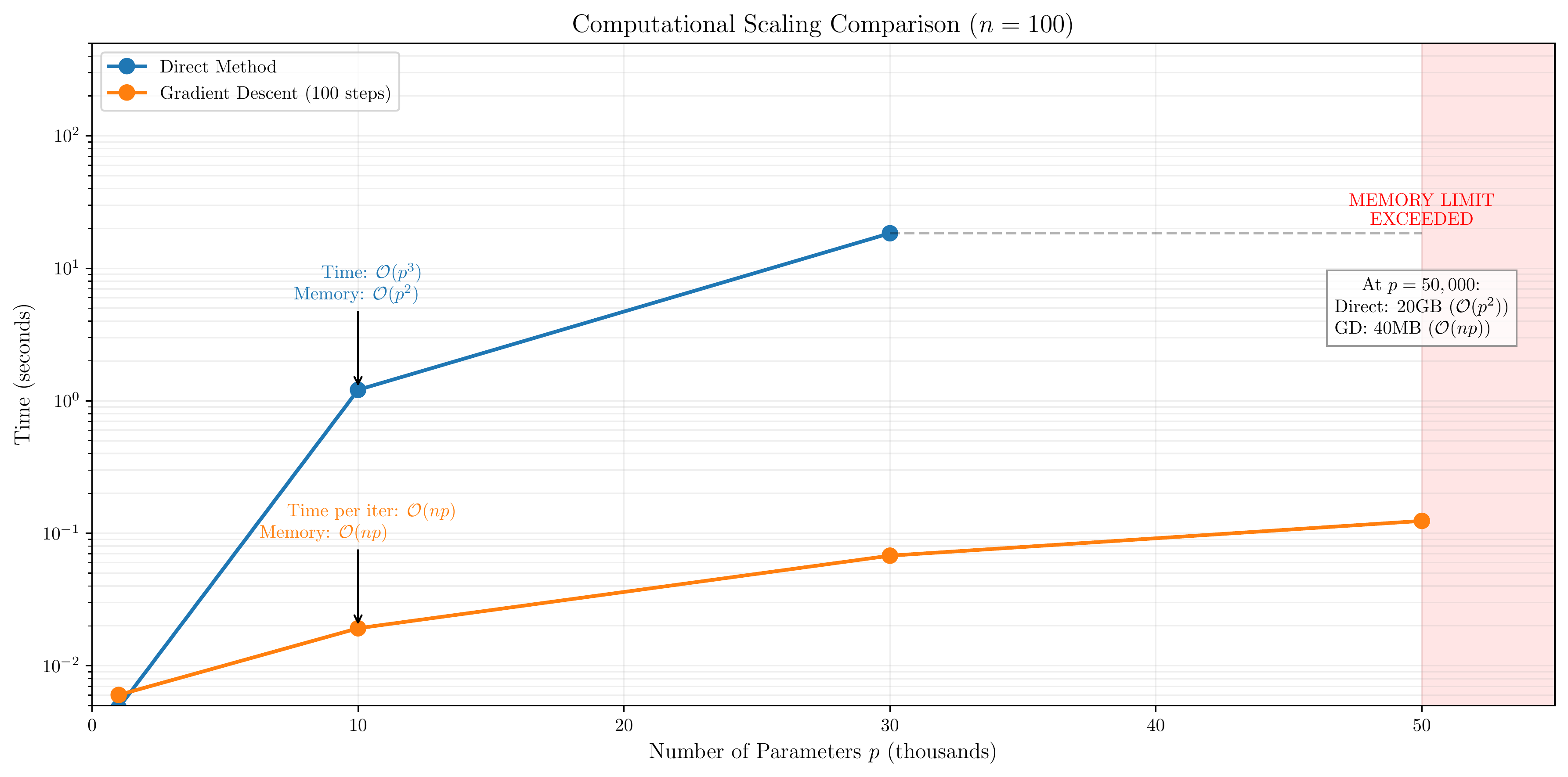
  • Figure 2.4: Memory/Compute scaling. Direct methods need $O(p^2)$ memory, GD needs $O(n)$ compute/step. SGD avoids these. (Lecture 3)
• SGD Solution: Use estimate $g(w_k)$ from mini-batch/sample: $w_{k+1} = w_k - \alpha g(w_k)$ (L6, L8).

Understanding SGD Behavior (via NQM etc.)

• Converges in expectation.
• Constant $\alpha \implies$ convergence to noise floor (steady-state error), size $\propto \alpha/B$ (L6, L7). Need decreasing $\alpha$ for exact convergence.
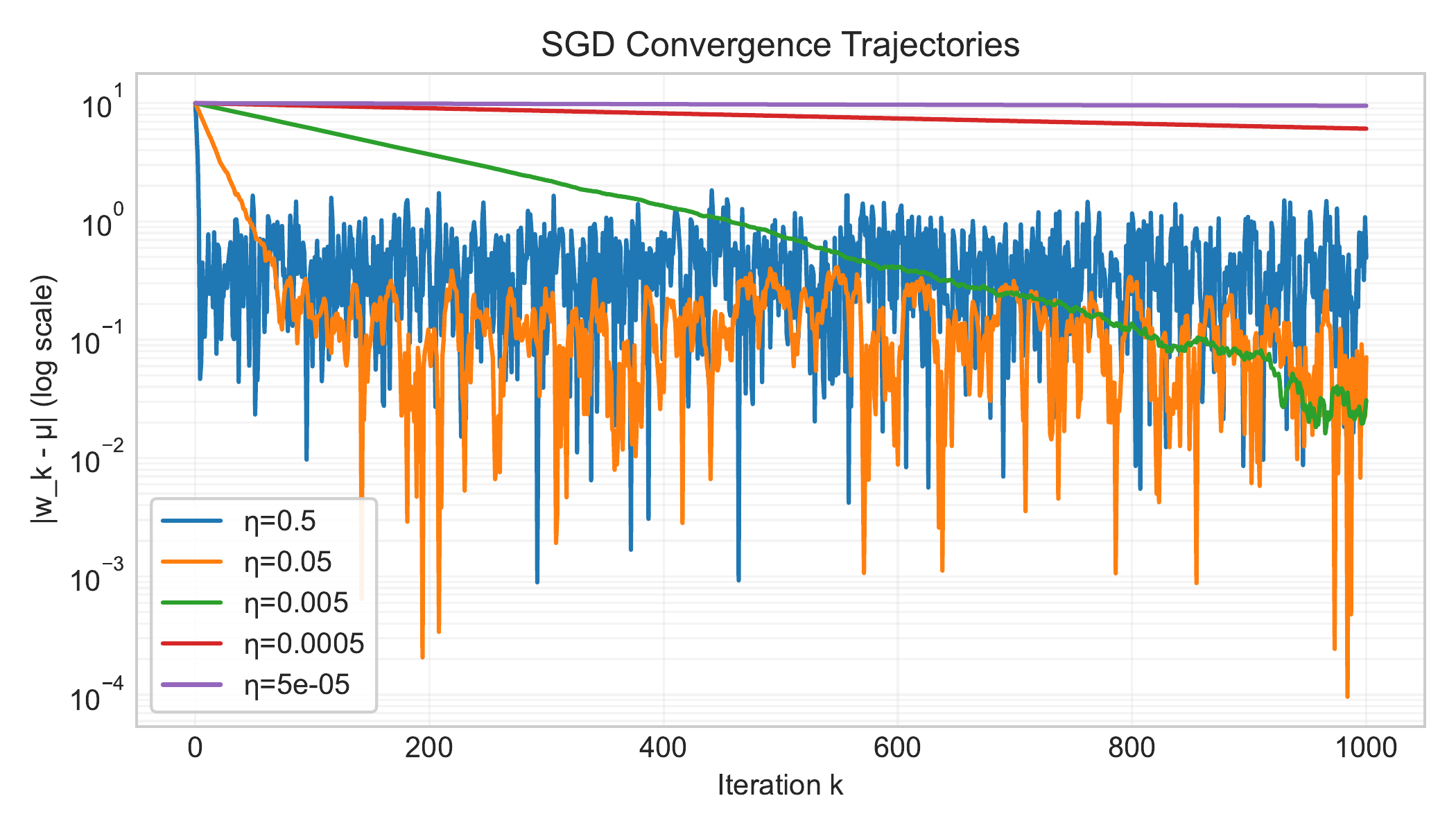
  • Figure 2.5: SGD noise floor with constant $\eta$. Error decreases then plateaus. (Lecture 6)
• Conditioning number $\kappa$ affects speed (L2, L3, L7). Poor conditioning $\implies$ slow convergence / oscillations.
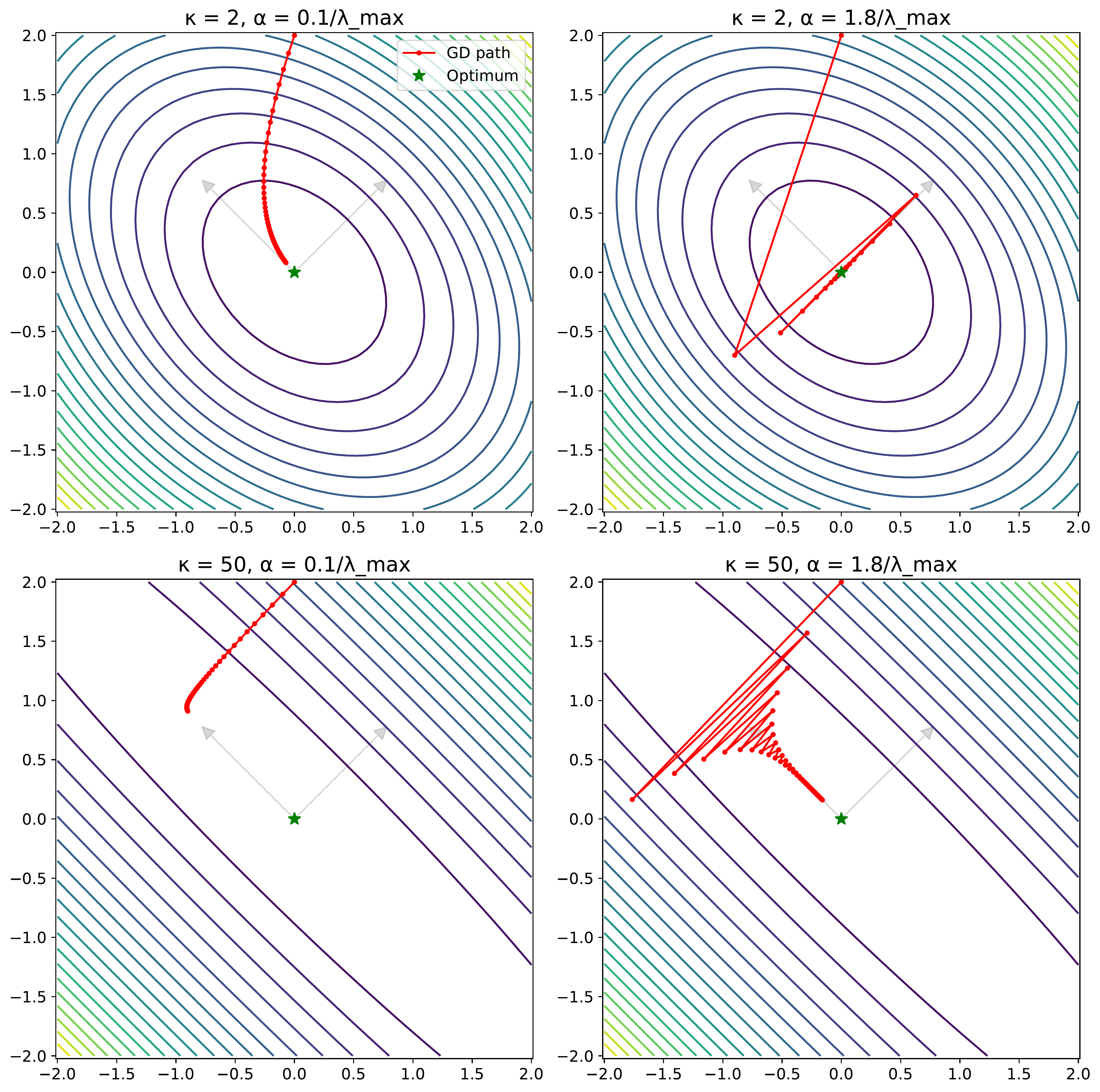
  • Figure 2.6: High conditioning ($\kappa=50$) causes GD to zigzag, especially with larger steps. (Lecture 3)

SGD Variants (Insights from NQM L7)

• Momentum: Reduces initial error (good for large B / low noise). Can increase noise floor.
• EMA: Reduces steady-state risk (good for small B / high noise). Minimal effect on initial rate.
• Preconditioning: Addresses poor conditioning $\kappa$ (good for large B). Can amplify noise.

Adaptive Methods & Practical Tools

• Adaptive Opt: Adagrad, Adam, AdamW adjust LR per parameter (L9). Useful for varied scales/complex landscapes.
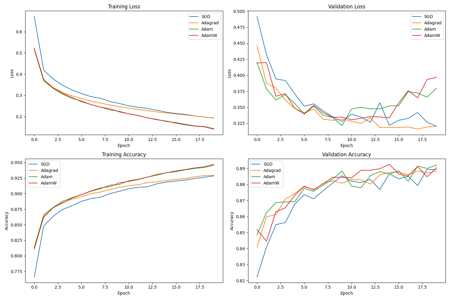
  • Figure 2.7: Adaptive methods (Adam/AdamW) often converge faster initially on tasks like Fashion MNIST. (Lecture 9)
• Standard Practice: Weight Decay (regularization) & Learning Rate Schedules are essential (L8).

Practical Tuning & Evaluation

• Process Matters: Systematic tuning (Deep Learning Tuning Playbook, L11). Incremental changes, Exploration > Exploitation, Scientific/Nuisance/Fixed parameters.
  • Figure 2.8: Iterative tuning workflow: structure exploration before exploitation. (Lecture 11)
• Fair Comparison: Optimizer comparisons depend heavily on the tuning protocol (space, budget) (L10). Use benchmarks, Time-to-Result metric. Key to being an intelligent consumer.
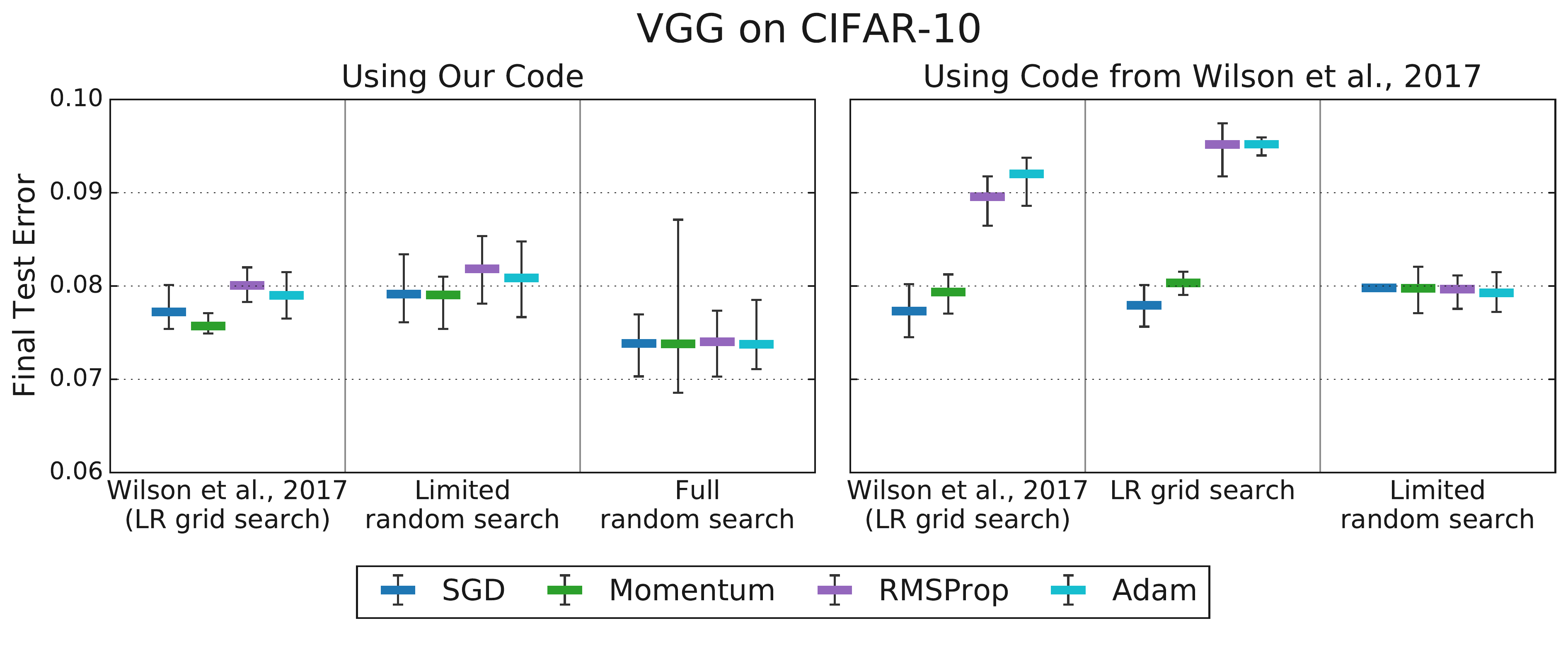
  • Figure 2.9: Tuning protocol matters! Differences seen with limited tuning vanish with fair, comprehensive tuning. (Choi et al. 2019b, L10)

Scaling Large Models (L12)

• Bottleneck: Activation Memory. Grows with batch size b, sequence length s.
• Solution 1: Activation Recomputation (Gradient Checkpointing) - trade compute for memory.
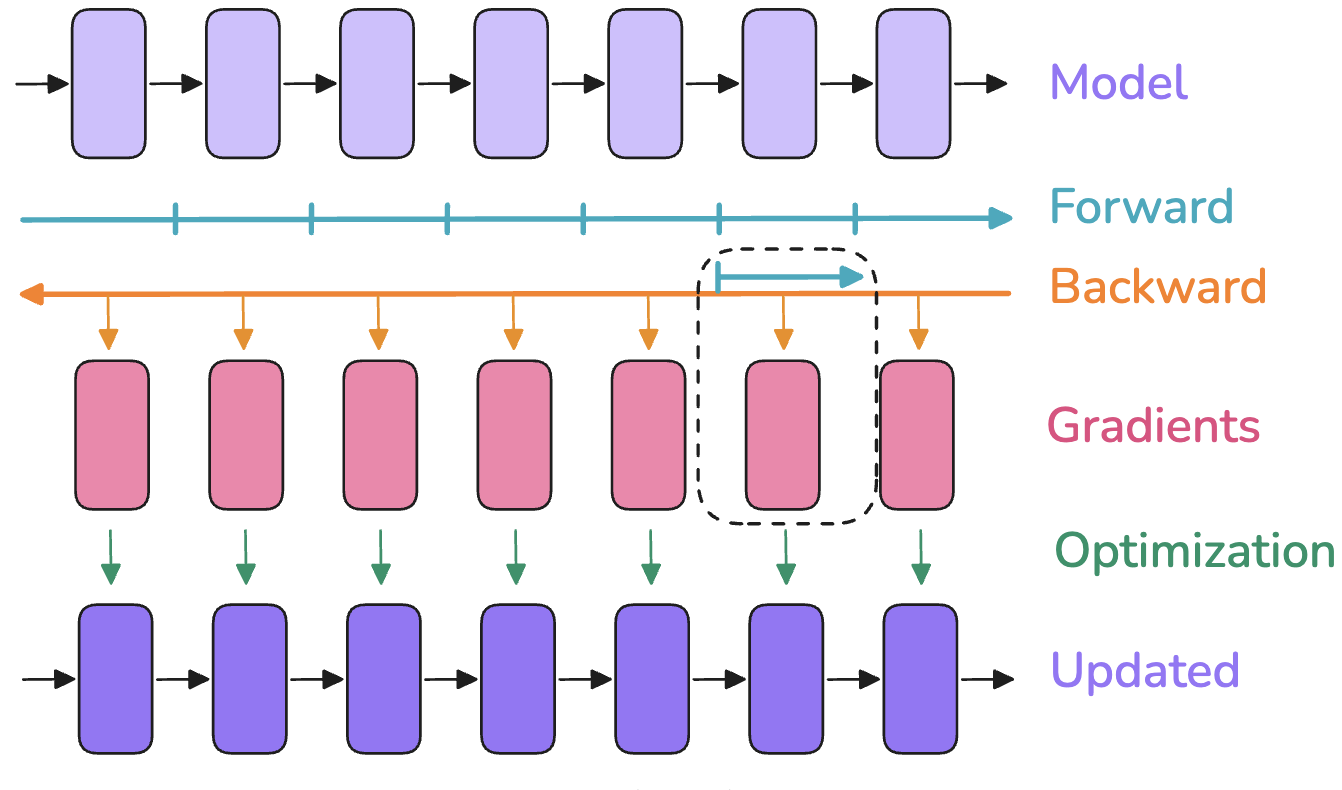
  • Figure 2.10: Recompute activations during backward pass instead of storing all. Saves memory. (Lecture 12)
• Solution 2: Parallelism Strategies. Combine:
  • Data Parallelism (DP / ZeRO / FSDP) - Replicate model, shard data/state.
  • Pipeline Parallelism (PP) - Shard layers across devices.
  • Tensor Parallelism (TP / SP) - Shard ops/tensors within layers.
  • Figure 2.11: Combining parallelism (DP, PP, TP etc.) is needed for state-of-the-art scale. (Lecture 12)

---

3. How Did We Measure Up? (Learning Outcomes from L0)

• Goal: Foster ability as an intelligent consumer of optimization methods.
• 1. Modeling & Formulation: Practiced framing ML problems as $L(w) = \frac{1}{n}\sum \ell(w, z_i)$. Project required this. Less focus on RL formulations in lectures. (Achieved, with caveats)
• 2. Algorithm Selection & Analysis: Covered SGD variants, Adam/W. Analyzed tradeoffs (NQM, conditioning). Discussed benchmarking. Quasi-Newton less covered. (Largely Achieved)
• 3. Software Proficiency: Heavy PyTorch focus (autograd, nn, optim). Project demanded implementation. (Core Achievement)
• 4. Optimization in Practice: Emphasized tuning playbook, practical hyperparameters (LR schedules, WD), evaluation. Less formal theory. (Core Achievement)
• 5. Research Methods: Discussed benchmarking. Project simulated research workflow. Scaling addressed constraints. Privacy/specific constraints not covered. (Partially Achieved)

---

4. What We Didn’t Cover

• Convex Optimization Theory: Formal properties, duality, detailed convergence rates, specialized solvers (CVXPY).
• Other Formulations: Compressive Sensing, Diffusion Models (in lectures).
• Reinforcement Learning (RL): Briefly introduced (L13 draft), but requires dedicated study.
• Advanced Opt Topics: Higher-order methods (Newton), Constrained Opt (Projections, Proximal), Privacy-Preserving Opt, Scaling Laws (MuP).

---

5. Where to Go From Here

• Coursework: Advanced Optimization (Convex), Reinforcement Learning, Domain-specific ML (NLP, Vision).
• Project: Refine course project $\rightarrow$ paper, portfolio, open-source.
• Theory: Textbooks (Boyd & Vandenberghe, Nocedal & Wright), research papers.
• Systems: Distributed computing, GPU programming (CUDA), large-scale training engineering.
• Contribute: Open-source libraries (PyTorch, Jax, Hugging Face).

---

6. Conclusion

• Core Message: Numerical optimization + PyTorch = powerful, practical framework for ML/Data Science. Aim: Become an intelligent consumer.
• Personal Note 1: Enjoyed high interaction via project meetings. Impressed by project ambition & diligence. Fun seeing concepts applied creatively.
• Personal Note 2: Enjoyed discussing practical optimization relevance (esp. for AI). Appreciated insightful questions. Potential for Part 2 course (Adv. Methods, RL).
• Personal Note 3: Course was experimental. Plan to refine/update for Spring 2026, streamlining content.
• Final Thanks: Thank you for your participation and effort.

---