Course Recap: Optimization in PyTorch

Cheatsheet

Table of Contents

1. Introduction
2. What We Learned: Key Concepts and Skills
3. How Did We Measure Up? Revisiting Learning Outcomes
4. What We Didn’t Cover
5. Where to Go From Here
6. Conclusion

1. Introduction

This lecture provides a final recap for Stat 4830. The objective is to consolidate the primary concepts and practical skills developed throughout the semester. This review will help solidify your understanding of the material covered.

The central theme of this course has been learning to formulate and solve numerical optimization problems relevant to modern data science and machine learning. We placed a strong emphasis on practical implementation using the PyTorch library. The semester-long project structure provided a consistent opportunity for hands-on application of these ideas. As stated in the course overview, the overall goal was: “By the end of this course, you will become an intelligent consumer of numerical methods and software for solving modern optimization problems.” This recap aims to reinforce the foundation needed to achieve that goal.

2. What We Learned: Key Concepts and Skills

We began with the fundamentals of PyTorch, starting with tensor creation and basic linear algebra operations (Lecture 1). A key step was understanding PyTorch’s automatic differentiation system, autograd (Lecture 4). We connected this mechanism back to the core ideas of calculus, viewing the derivative or Jacobian as the best linear approximation of a function and autograd as an efficient implementation of the chain rule (Lecture 5).

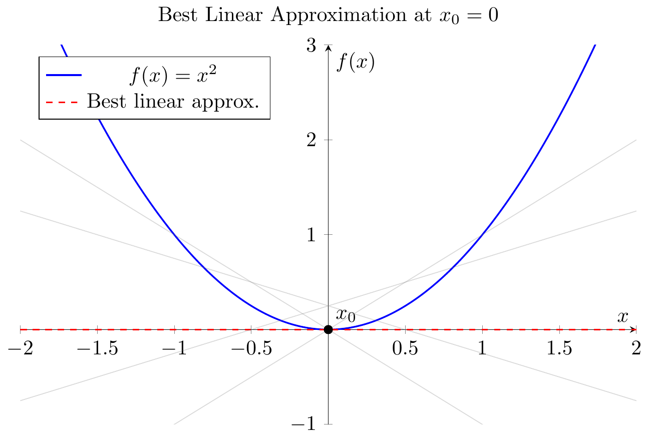Figure 2.1: The derivative as the best linear approximation. The tangent line $L(x) = f(a) + f’(a)(x-a)$ provides the closest linear fit to $f(x)$ near $x=a$. (Lecture 5)

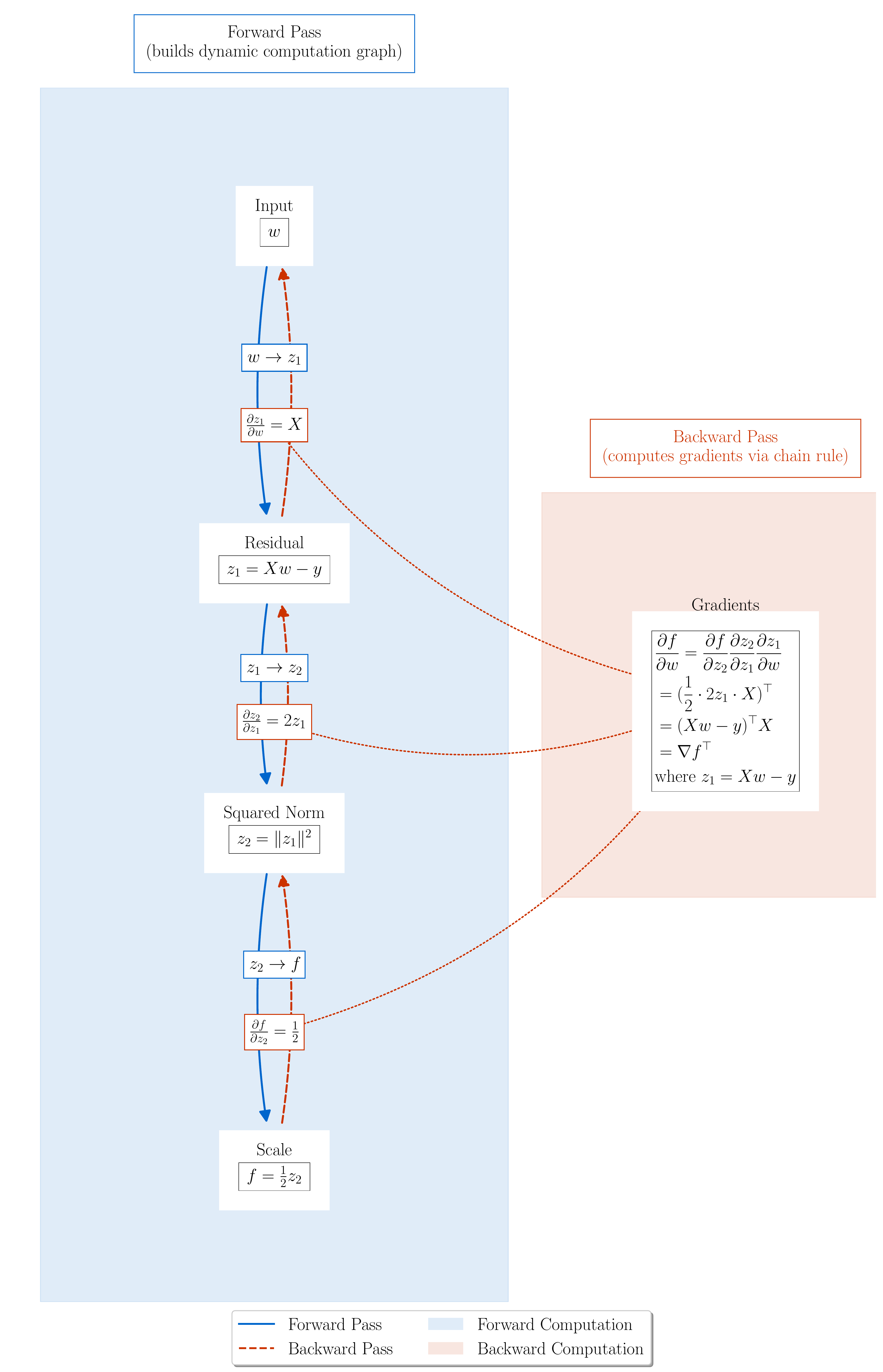Figure 2.2: Computational graph for Least Squares loss $L(w) = \frac{1}{2}|Xw - y|^2$. autograd builds this graph during the forward pass and uses it to compute gradients via the chain rule during backward(). (Lecture 4)

We then saw how to use standard PyTorch components like nn.Module to define model architectures, DataLoader to manage data batches, torch.optim to apply optimization algorithms, and torch.optim.lr_scheduler to adjust learning rates during training (Lecture 8).

These tools allowed us to frame common machine learning tasks as optimization problems. We consistently represented the goal as minimizing an objective function $L(w)$, typically an average loss over training data, $L(w) = \frac{1}{n}\sum_{i=1}^n \ell(w, z_i)$. Examples included linear regression using squared error loss, $\ell(w, x_i, y_i) = \frac{1}{2}(w^T x_i - y_i)^2$ (Lecture 2, Lecture 3), and classification problems often addressed with cross-entropy loss (Lecture 0, Lecture 4).

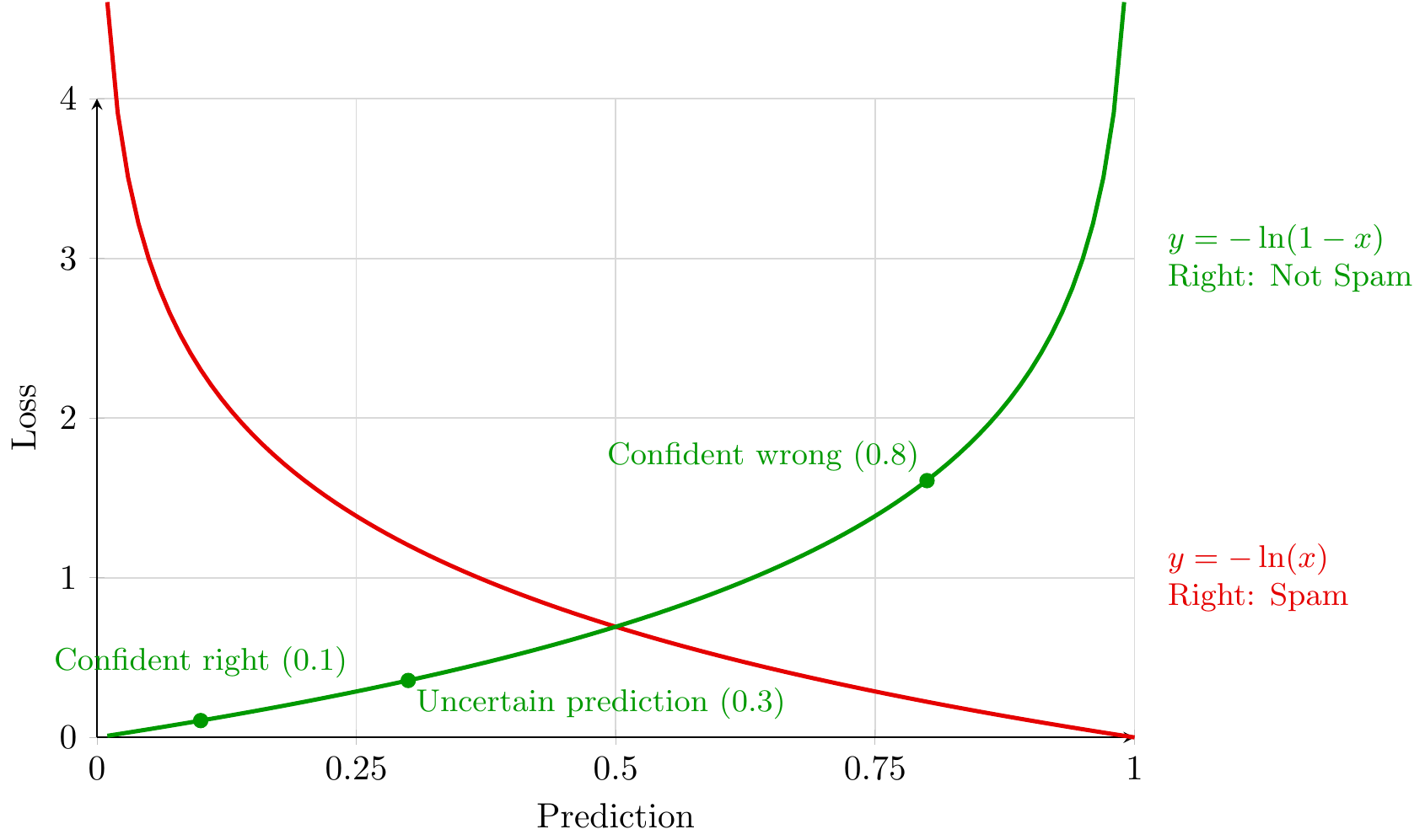Figure 2.3: Cross-entropy loss penalizes incorrect predictions, especially confident ones, guiding classification models. (Lecture 0)

We studied the standard gradient descent update rule, $w_{k+1} = w_k - \alpha \nabla L(w_k)$ (Lecture 3). The main computational challenge identified was the cost of computing the full gradient $\nabla L(w)$, which requires iterating through all $n$ data samples. For large datasets, this is impractical. Stochastic Gradient Descent (SGD) was introduced as the necessary alternative, using updates based on gradient estimates $g(w_k)$ derived from small mini-batches or single samples: $w_{k+1} = w_k - \alpha g(w_k)$ (Lecture 6, Lecture 8).

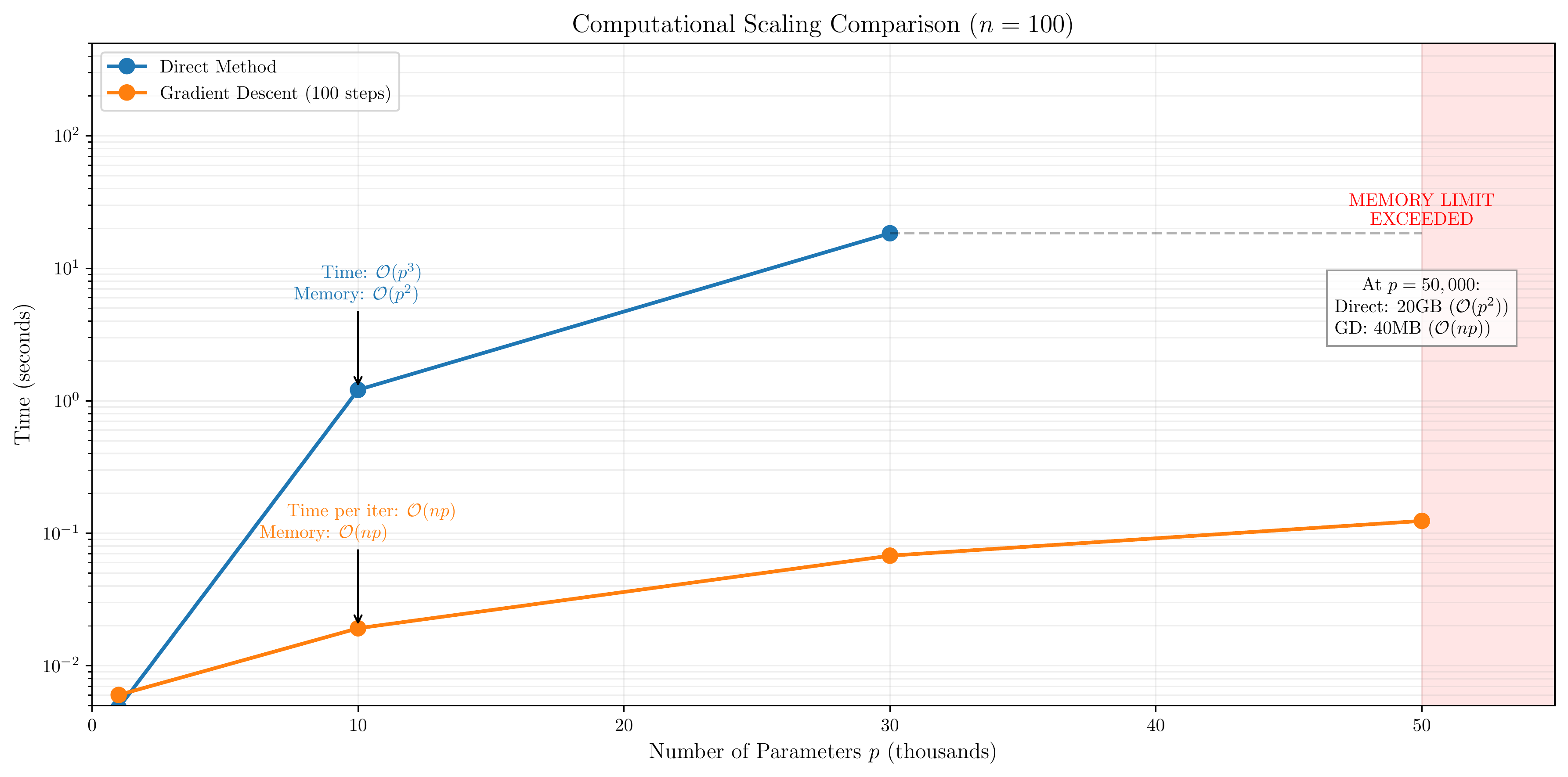Figure 2.4: Memory scaling comparison for direct methods vs. gradient descent. Forming $X^T X$ has $O(p^2)$ memory cost, becoming a bottleneck before the $O(p^3)$ compute cost for solving. Gradient descent avoids this via matrix-vector products with $O(np)$ cost and $O(p)$ memory per step. (Lecture 3)

Analyzing SGD’s behavior, particularly through simplified models like mean estimation (Lecture 6) and the Noisy Quadratic Model (NQM) (Lecture 7), revealed key properties. With a constant learning rate $\alpha$ and batch size $B$, SGD converges in expectation. However, it does not converge to the exact optimum but rather to a “noise floor” or steady-state error region whose size is influenced by $\alpha/B$. We also reinforced the importance of the problem’s conditioning number $\kappa$ (Lecture 2, Lecture 3) as a factor affecting convergence speed for both gradient descent and SGD (Lecture 7). Achieving high precision with SGD necessitates reducing the learning rate over time.

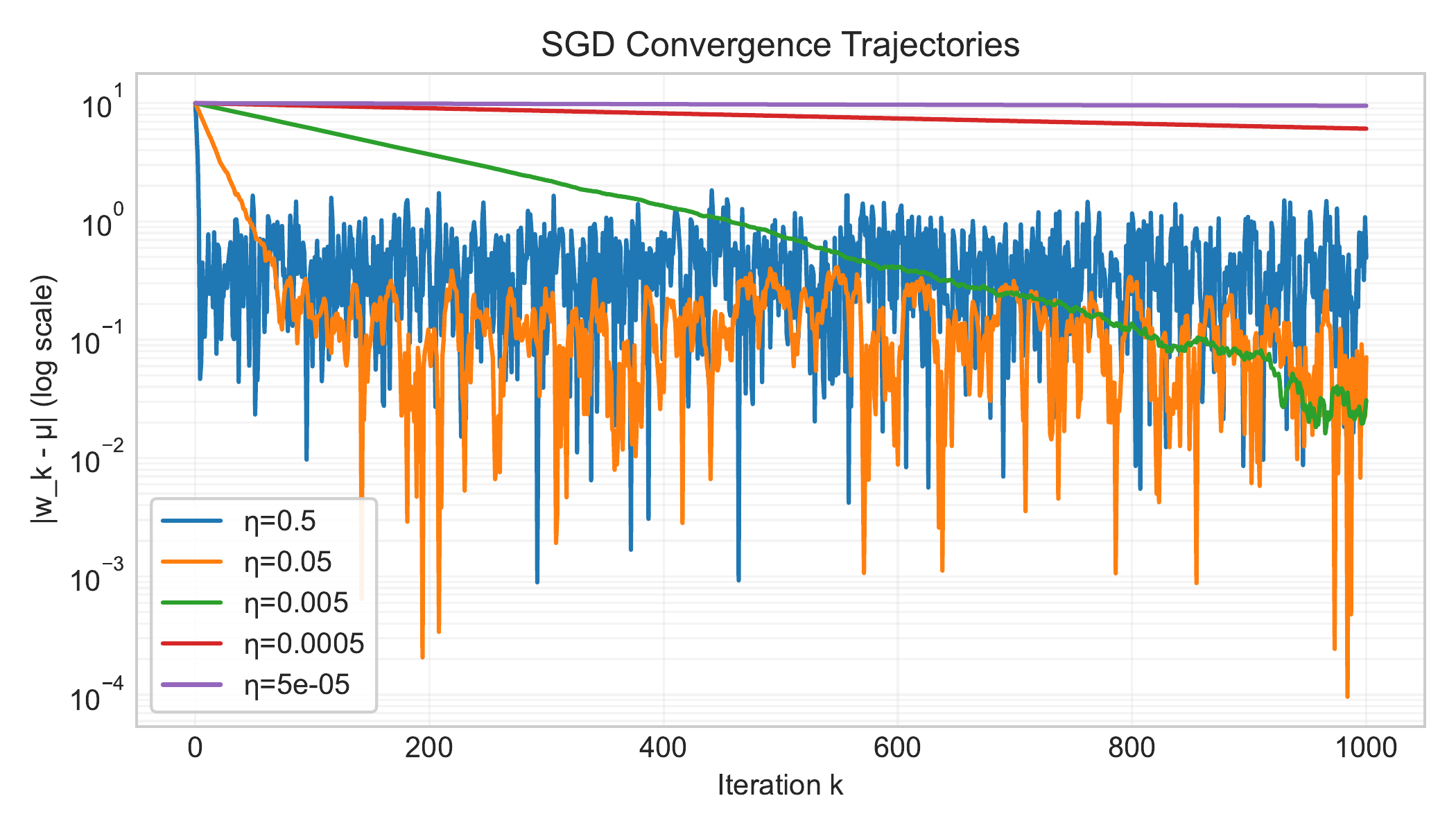Figure 2.5: Convergence of SGD iterates for mean estimation. With constant step size $\eta$, the error decreases initially but then fluctuates around a non-zero noise floor. Smaller $\eta$ leads to a lower noise floor but slower initial convergence. (Lecture 6)

We also reinforced the importance of the problem’s conditioning number $\kappa$ (Lecture 2, Lecture 3) as a factor affecting convergence speed for both gradient descent and SGD (Lecture 7). Poor conditioning ($\kappa \gg 1$) leads to slow convergence, often characterized by oscillations.

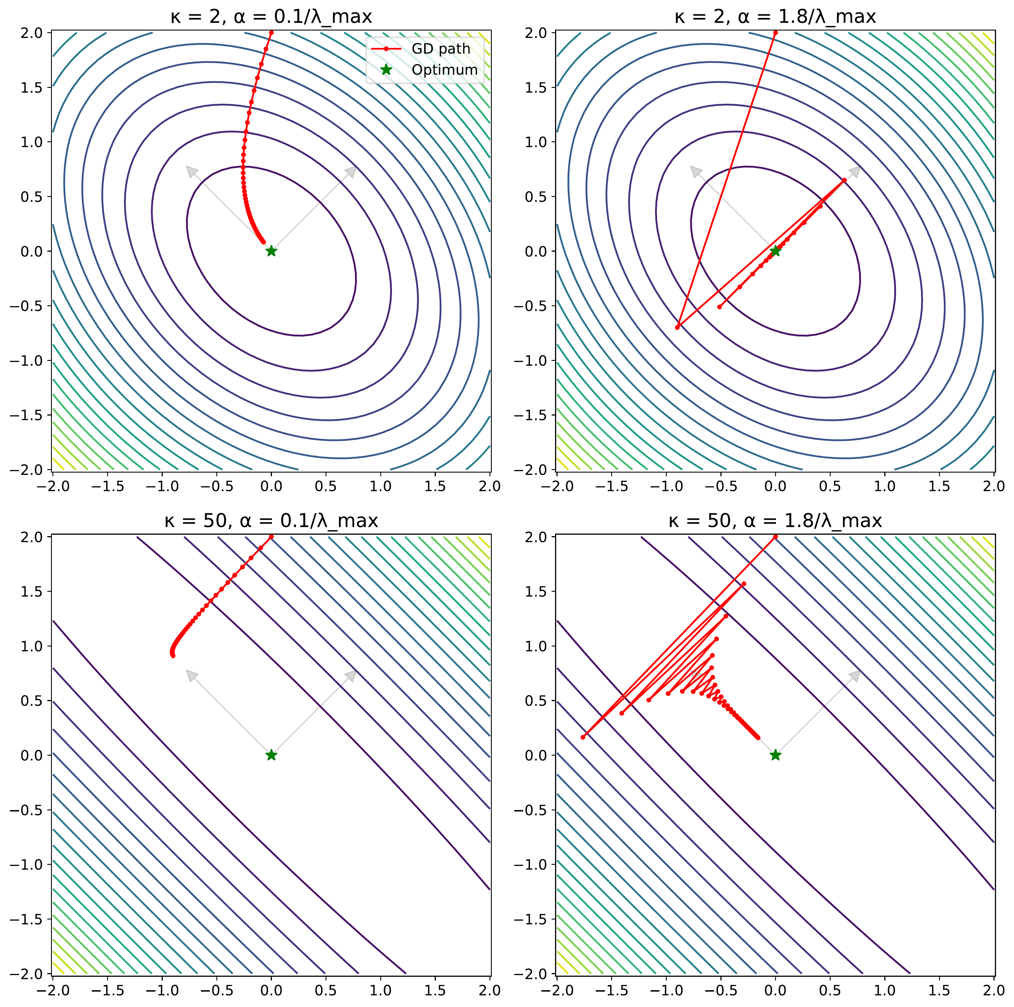Figure 2.6: Effect of conditioning ($\kappa$) and step size ($\alpha$) on gradient descent paths. High conditioning ($\kappa=50$, bottom row) causes zigzagging, especially with larger steps, as the algorithm navigates elongated loss contours. (Lecture 3)

The NQM analysis (Lecture 7) also provided insights into the roles of common SGD variants in that specific context. Momentum was shown to primarily help reduce initial error, making it beneficial in low-noise (large batch size) settings, though potentially increasing the noise floor. Exponential Moving Average (EMA) was shown to primarily reduce the steady-state risk, making it useful in high-noise (small batch size) settings. Preconditioning helps address poor conditioning, accelerating convergence particularly in large-batch scenarios, but can also amplify noise.

Beyond basic SGD modifications, we introduced adaptive methods like Adagrad, Adam, and AdamW (Lecture 9). These algorithms adjust the learning rate for each parameter automatically, which can be helpful for problems with varying feature scales or complex loss landscapes. We also discussed Weight Decay and Learning Rate Schedules (Lecture 8) not just as theoretical concepts, but as standard tools essential for achieving good performance in practical deep learning training.

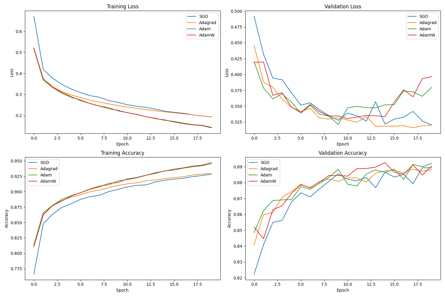Figure 2.7: Performance comparison on Fashion MNIST. Adaptive methods (Adam, AdamW) often show faster initial progress compared to SGD+Momentum, though final performance depends heavily on tuning. (Lecture 9)

Moving from algorithms to application, the course emphasized the process of optimization. The Deep Learning Tuning Playbook (Lecture 11) provided a framework for systematic tuning: making incremental changes, differentiating between exploration (seeking understanding) and exploitation (maximizing performance), and managing scientific versus nuisance hyperparameters.

Figure 2.8: Overview of the iterative tuning process based on the Deep Learning Tuning Playbook. Emphasizes structured exploration and evidence-based decisions. (Lecture 11)

We also discussed the challenges of reliably comparing optimizer performance (Lecture 10), stressing the importance of the tuning protocol itself and the utility of standardized benchmarks using metrics like Time-to-Result. Understanding how to tune and evaluate methods is key to being an intelligent consumer.

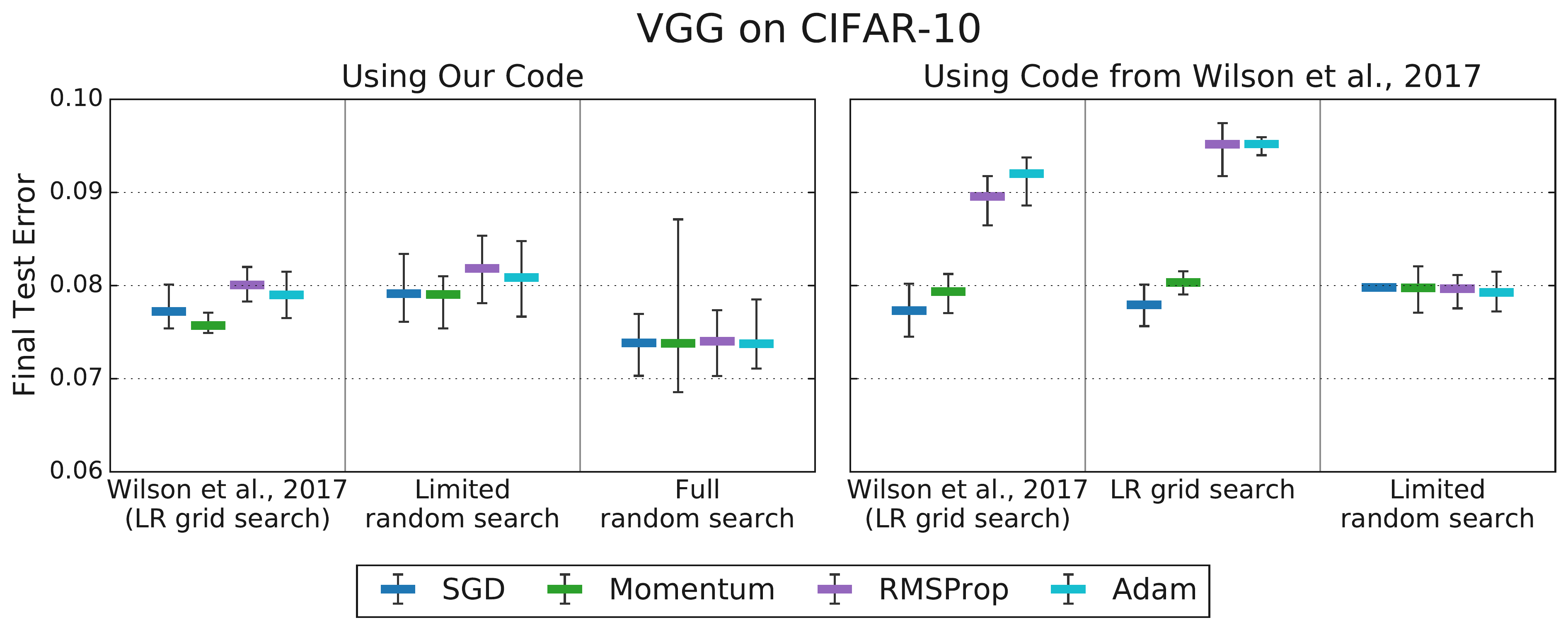Figure 2.8: The effect of tuning protocol (from Choi et al., 2019b). Limited tuning (left) can suggest performance differences between optimizers that disappear with more comprehensive, fair tuning (right), highlighting the protocol’s importance. (Lecture 10)

Finally, we touched upon the challenges of training extremely large models (Lecture 12). We identified activation memory as a primary bottleneck during backpropagation and introduced activation recomputation (gradient checkpointing) as a technique to trade compute for memory.

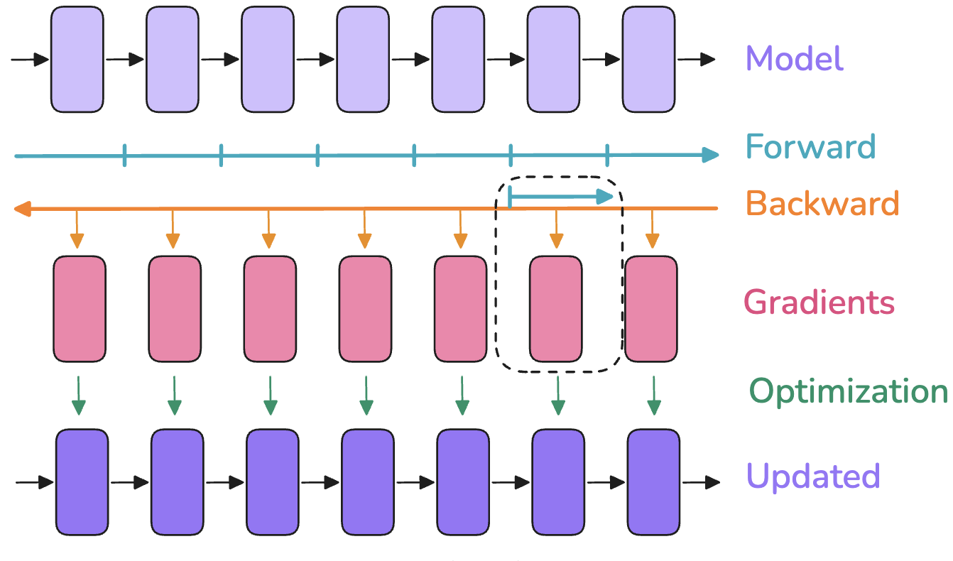Figure 2.9: Activation Recomputation. Instead of storing all intermediate activations (top), only store checkpoints (e.g., layer inputs) and recompute activations within a segment during the backward pass (bottom), saving memory at the cost of extra forward computation. (Lecture 12)

We listed the main parallelism strategies—Data Parallelism (DP/FSDP), Pipeline Parallelism (PP), and Tensor Parallelism (TP/SP)—used to distribute the computation and model state across multiple devices, noting that combining these strategies is typically required for state-of-the-art scale.

Figure 2.11: Conceptual Overview of Combined Parallelism Dimensions (DP, PP, TP, EP, CP). Large-scale training often requires combining multiple strategies. (Lecture 12)

3. How Did We Measure Up? Revisiting Learning Outcomes

We now briefly review the learning outcomes stated in the syllabus (Lecture 0) at the beginning of the course. This reflection helps assess how the material covered aligns with the initial goals for what you would be able to do after completing Stat 4830. The aim remains to foster your ability to be an “intelligent consumer” of numerical optimization methods.

The first outcome was: “Modeling and Formulation - By the end of this course, you should be able to take a real-world problem (in data science, machine learning, or sequential decision-making) and translate it into a formal optimization problem with well-defined objectives and constraints.” We practiced formulating problems like classification and regression as minimizing an average loss $L(w) = \frac{1}{n}\sum \ell(w, z_i)$ (Lecture 0, Lecture 2). The course project required you to undertake this modeling step for your chosen application. While lecture coverage of sequential decision-making formulations was limited, the core principle of defining an objective $L(w)$ applies broadly.

The second outcome focused on: “Algorithm Selection and Analysis - You will learn how to choose an appropriate algorithm—from basic gradient descent to more advanced quasi-Newton methods—and understand the trade-offs of different approaches (speed, accuracy, scalability).” We covered SGD and its variants, including momentum and adaptive methods like Adam and AdamW (Lectures 6-9). Our analysis using models like the NQM (Lecture 7) provided a framework for understanding trade-offs related to noise, conditioning $\kappa$, and batch size. Benchmarking discussions (Lecture 10) addressed comparing methods based on speed and accuracy. Coverage of quasi-Newton methods was minimal.

The third outcome was: “Software Proficiency - We will use modern libraries like PyTorch (possibly Jax) to implement and experiment with these algorithms. You will gain experience with auto differentiation and learn best practices for tuning and debugging iterative solvers.” PyTorch proficiency was a central objective. We progressed from basic tensor manipulation (Lecture 1) through the mechanics of autograd (Lecture 4, Lecture 5) to implementing optimization loops using torch.optim (Lecture 8). The course project served as the primary vehicle for gaining hands-on implementation and debugging experience.

The fourth outcome concerned: “Optimization in Practice - Although we’ll cover fundamental optimization theory (convexity, convergence rates, saddle points, etc.), the focus is on practical usage. You will learn which methods to try first and how to iterate quickly when working with large datasets and complicated models.” The course strongly emphasized practical usage. We covered practical hyperparameter considerations like learning rate schedules and weight decay (Lecture 8), the systematic tuning process outlined in the Deep Learning Tuning Playbook (Lecture 11), and methods for evaluating performance (Lecture 10). The project work necessitated iterating on practical optimization problems. Less time was spent on formal optimization theory compared to a traditional course.

The final outcome was: “Research Methods - This course also prepares you for research or advanced development tasks. You’ll see how to benchmark optimization methods, reproduce existing studies, and innovate ways to handle constraints like privacy and distributed data.” We discussed benchmarking methodologies for comparing optimizers (Lecture 10). The project, structured around regular progress reports and culminating in a final report and implementation, simulated aspects of a research workflow. Several projects involved reproducing or extending results from the literature. The lecture on scaling (Lecture 12) touched upon handling computational constraints common in research. Specific topics like privacy-preserving methods were not covered in lectures.

4. What We Didn’t Cover

Given the available time and the course’s focus on practical implementation in PyTorch, several relevant topics in optimization were covered briefly or not at all. This section acknowledges some of those areas.

We did not delve deeply into the theory of Convex Optimization. While convexity was mentioned (Lecture 0, Lecture 3), we did not explore the formal properties of convex functions and sets, duality theory, or the specialized algorithms and convergence guarantees associated with convex problems. Software like CVXPY, designed for convex problems, was introduced (Lecture 0) but not used extensively in our PyTorch-centric approach.

Certain specific Optimization Formulations prominent in other fields or advanced machine learning were not covered in lectures. Examples include methods used in signal processing like compressive sensing or optimization problems arising in training generative models like diffusion models, although some course projects explored related areas.

Reinforcement Learning (RL) represents a vast field involving sequential decision-making problems formulated using MDPs (Lecture 13). While introduced, the algorithmic depth required to cover RL effectively was beyond the scope achievable in this course structure. The draft notes for Lecture 13 offer a starting point for those interested.

Finally, several Advanced Optimization Topics listed as potential areas in the syllabus were omitted. These include higher-order optimization methods (like Newton or quasi-Newton methods), techniques for handling constrained optimization problems (such as projections or proximal operators), methods for privacy-preserving optimization (like differential privacy), and theoretical frameworks for predicting large model performance (like scaling laws).

5. Where to Go From Here

The concepts and skills covered in this course provide a foundation for several future directions. For those interested in further coursework, seeking out advanced classes in optimization, particularly convex optimization, would deepen theoretical understanding. Dedicated courses on reinforcement learning or specialized machine learning domains like natural language processing or computer vision would allow you to apply these optimization techniques to specific problem areas.

Your work on the course project offers another avenue. Consider refining your project further; it could potentially evolve into a research paper, a demonstration for job applications, or even an open-source contribution.

If you are interested in theory, standard textbooks like Boyd and Vandenberghe’s “Convex Optimization” or Nocedal and Wright’s “Numerical Optimization” offer comprehensive treatments. Reading and reproducing results from research papers on optimization algorithms and their convergence properties is another way to engage more deeply.

For those interested in the systems aspect, exploring distributed computing, GPU programming frameworks like CUDA, and the software engineering challenges involved in training large-scale models (Lecture 12) are relevant next steps.

Finally, contributing to open-source machine learning libraries is a practical way to apply and enhance your skills. Libraries associated with PyTorch, Jax, or platforms like Hugging Face often involve optimization components and welcome contributions from the community.

6. Conclusion

Numerical optimization provides a powerful and practical framework for addressing problems across data science and machine learning. This course aimed to equip you with the understanding and tools, particularly within the PyTorch ecosystem, needed to effectively apply these methods. Hopefully, the material covered, from fundamental concepts like automatic differentiation to the analysis of stochastic gradient methods and the practicalities of tuning and scaling, has moved you closer to becoming an intelligent consumer and practitioner of numerical optimization techniques.

On a personal note, one very rewarding aspect of this course was the opportunity for regular interaction through the project meetings. I genuinely enjoyed our bi-weekly discussions and seeing the ambition and diligence you brought to your projects. It was impressive to watch you creatively apply the optimization concepts we discussed to your diverse research interests.

Discussing the practical side of optimization, especially its crucial role in the current landscape of artificial intelligence, was also enjoyable. Your questions throughout the semester were insightful and contributed to a positive learning environment. There is certainly more ground to cover! In an ideal world, I would teach a part 2 of this course exploring advanced numerical methods for machine learning and reinforcement learning further.

This course was an initial offering, and I see opportunities for refinement. I plan to teach an updated version in Spring 2026. The field changes rapidly; while core optimization principles will remain, the specific content will likely evolve. I aim to streamline the material to focus efficiently on the most useful concepts.

Thank you for your participation and effort in this course.